r


29
Jun 10

Entropy augmentation the modulo way

Long before I had heard about the connection between entropy and probability theory, I knew about it from the physical sciences. This is most likely how you met it, too. You heard that entropy in the universe is always increasing, and, if you’re like me, that made very little sense. Then you may have heard that entropy is a measure of disorder: over times things fell apart. This makes a little more sense, especially to those teenagers tasked with cleaning their own rooms. Later on, perhaps you got a more precise, mathematical definition of entropy that still didn’t fully mesh with the world as we observe it. Here on earth, we see structures getting built up over time: plants convert raw energy to sunflowers, bees build honeycombs, humans build roads. Things do sometimes fall apart. More precisely, levels of complexity tend to grow incrementally over long periods of time, then collapse very quickly. This particular asymmetry seems to be an ironclad rule for our word, which I assume everyone understands, at least implicitly, though I can’t remember anywhere this rule is written down as such.

In the world of probability, entropy is a measure of unpredictability. Claude Shannon, who created the field of Information Theory, gave us an equation to measure how much, or little, is known about an incoming message a prori. If we know for sure exactly what the message will be, our entropy is 0. There is no uncertainty. If we don’t know anything about the outcome except that it will be one of a finite number of possibilities, we should assume uniform probability for any one of the outcomes. Uncertainty, and entropy, is maximized. The more you look into the intersection of entropy and statistics, the more you find surprising, yet somehow obvious in retrospect, connections. For example, among continuous distributions with fixed mean and standard deviation, the Normal distribution has maximal entropy. Surprised? Think about how quickly a sum of uniformly distributed random variables converges to the Normal distribution. Better yet, check it out for yourself:

n = 4
tally = rep(0,10000)
for(i in 1:n) {
	tally = tally + runif(10000)
}

hist(tally, breaks=50, col="blue")

Try increasing and decreasing “n” and see how quickly the bell curve begins to appear.

Lately I’ve been thinking about how to take any general distribution and increase the entropy. The method I like best involves chopping off the tails and “wrapping” these extreme values back around to the middle. Here’s the function I created:

smartMod <- function(x, mod) {
	sgn = sign(x)
	x = abs(x)
	x = x %% mod
	return(sgn * x)
}

Now is a perfect time to use a version of our “perfect sample” function:

perfect.sample <- function(dist, n, ...) {
	match.fun(paste('q', dist, sep=''))((1:n) / (n+1), ...)
}

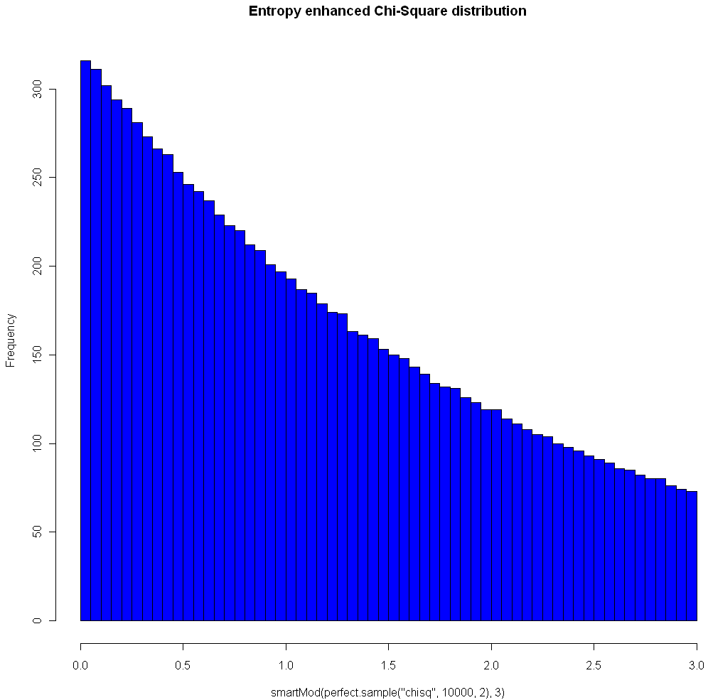
The image at the top of this post shows the Chi Square distribution on 2 degrees of freedom, with Modulo 3 Entropy Enhancement (see how nice that sounds?). Here’s the code to replicate the image:

hist(smartMod(perfect.sample("chisq",10000,2),3),breaks=70,col="blue",main="Entropy enhanced Chi-Square distribution")

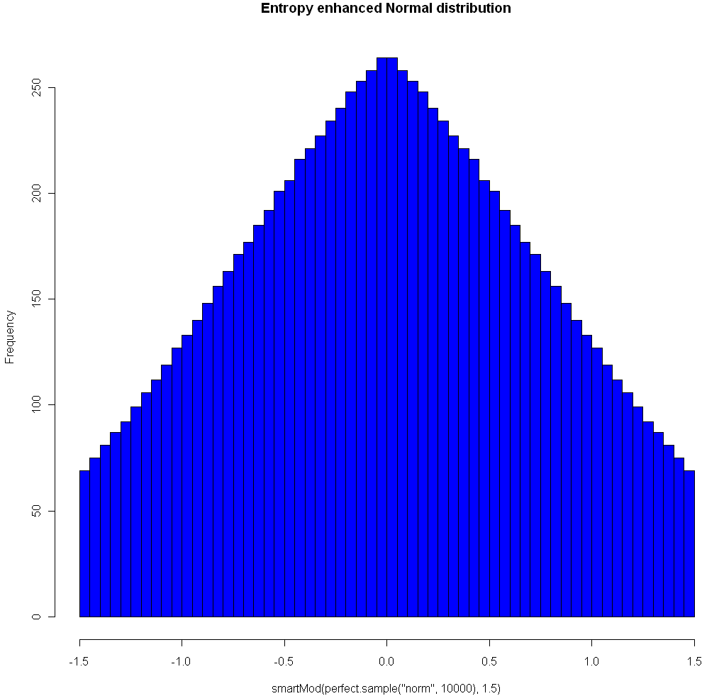
Here’s another plot, using the Normal distribution and Modulo 1.5:

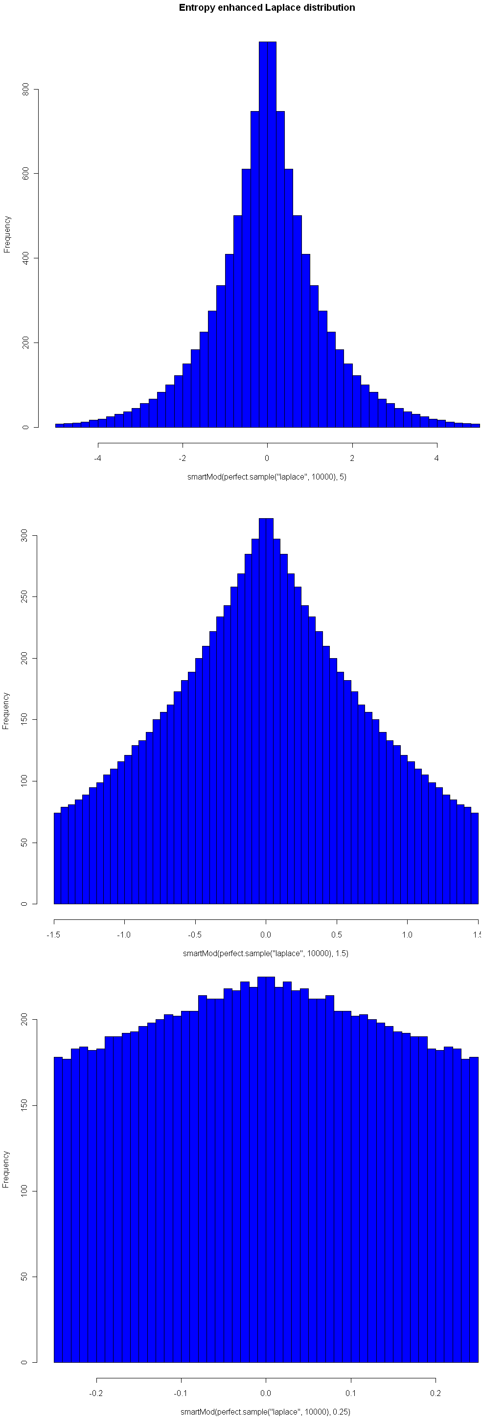
One nice property of this method of increasing entropy is that you get a smooth transition with logical extremes: As your choice of Mod goes to infinity, the distribution remains unchanged. As your Mod number converges to 0, entropy (for that given width) is maximized. Here are three views of the Laplace, with Mods 5, 1.5, and 0.25, respectively. See how nicely it flattens out? (Note you will need the library “VGAM” to sample from the Laplace).

It’s not clear to me yet how entropy enhancement could be of practical use. But everyone loves enhancements, right? And who among us doesn’t long for a  little extra entropy for time to time, no?


26
Jun 10

Weekend art in R (Part 2)

I put together four of the best looking images generated by the code shown here:

# More aRt
par(bg="white")
par(mar=c(0,0,0,0))
plot(c(0,1),c(0,1),col="white",pch=".",xlim=c(0,1),ylim=c(0,1))
iters = 500
for(i in 1:iters) {
	center = runif(2)
	size = 1/rbeta(2,1,3)
 
	# Let's create random HTML-style colors
	color = sample(c(0:9,"A","B","C","D","E","F"),12,replace=T)
	fill = paste("#", paste(color[1:6],collapse=""),sep="")
	brdr = paste("#", paste(color[7:12],collapse=""),sep="")
 
	points(center[1], center[2], col=fill, pch=20, cex=size)
	points(center[1], center[2], col=fill, pch=21, cex=size,lwd=runif(1,1,4))
}

Weekend art Part 1 is here.


22
Jun 10

Reaching escape velocity

Sample once from the Uniform(0,1) distribution. Call the resulting value [latex]x[/latex]. Multiply this result by some constant [latex]c[/latex]. Repeat the process, this time sampling from Uniform(0, [latex]x*c[/latex]). What happens when the multiplier is 2? How big does the multiplier have to be to force divergence. Try it and see:

iters = 200
locations = rep(0,iters)
top = 1
multiplier = 2
for(i in 1:iters) {
	locations[i] = runif(1,0,top)
	
	top = locations[i] * multiplier
}

windows()
plot(locations[1:i],1:i,pch=20,col="blue",xlim=c(0,max(locations)),ylim=c(0,iters),xlab="Location",ylab="Iteration")

# Optional save as movie, not a good idea for more than a few hundred iterations. I warned you!
# library("animation")
# saveMovie(for (i in 1:iters) plot(locations[1:i],1:i,pch=20,col="blue",xlim=c(0,max(locations)),ylim=c(0,iters),xlab="Location",ylab="Iteration"),loop=1,interval=.1)

19
Jun 10

The perfect fake

Usually when you are doing Monte Carlo testing, you want fake data that’s good, but not too good. You may want a sample taken from the Uniform distribution, but you don’t want your values to be uniformly distributed. In other words, if you were to order your sample values from lowest to highest, you don’t want them to all be equidistant. That might lead to problems if your underlying data or model has periods or cycles, and in any case it may fail to provide correct information about what would happen with real data samples.

However, there are times when you want the sample to be “perfect”. For example, in systematic sampling you may wish to select every 10th object from a population that is already ordered from smallest to biggest. This method of sampling can reduce the variance of your estimate without introducing bias. Generating the numbers for this perfect sample is quite easy in the case of the Uniform distribution. For example, R gives you a couple easy ways to do it:

# Generate a set of 100 equidistant values between 5 and 10 (inclusive)
x <- seq(5,10,length=100)

# Generate every 12th integer between 50 and 1000
x <- seq(50,1000,12)

When it comes to other distributions, grabbing a perfect sample is much harder. Even people who do a lot of MC testing and modeling may not need perfect samples every day, but it comes up often enough that R should really have the ability to do it baked right into to the language. However, I wasn't able to find such a function in R or in any of the packages, based on my searches at Google and RSeek. So what else could I do but roll my own?

# Function returns a "perfect" sample of size n from distribution myDist
# The sample is based on uniformly distributed quantiles between 0 and 1 (exclusive)
# If the distribution takes additional parameters, these can be specified in the vector params
# Created by Matt Asher of StatisticsBlog.com
perfect.sample <- function(n, myDist, params = c()) {
	x <- seq(0,1,length=(n+2))[2:(n+1)]
	  
	if(length(params)) {
	  	toEval <- paste(c("sapply(x,q", myDist, ",", paste(params,collapse=","), ")"), collapse="")
	} else {
	  	toEval <- paste(c("sapply(x,q", myDist, paste(params,collapse=","), ")"), collapse="")
	} 
	
	eval(parse(text=toEval))
}

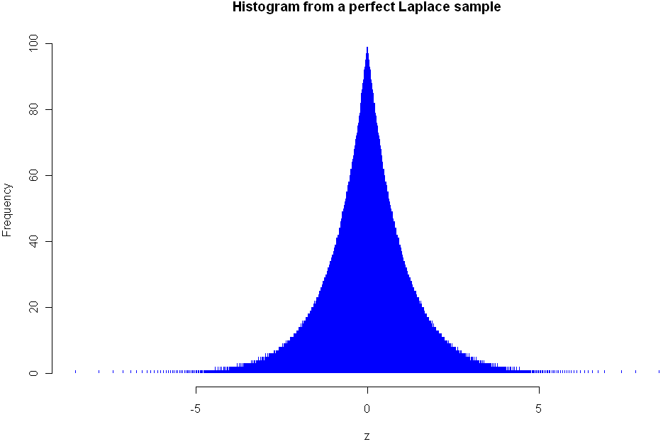
This function should work with any distribution that follows the naming convention of using "dname" for the density of the distribution and has as its first parameter the number of values to sample. The histogram at the top of this post shows the density of the Lapalce, aka Double Exponential distribution. Here is the code I used to create it:

# Needed library for laplace
library(VGAM)
z <- perfect.sample(5000,"laplace",c(0,1))
hist(z,breaks=800,col="blue",border=0,main="Histogram from a perfect Laplace sample")

As you can see, my function plays nice with distributions specified in other packages. Here are a couple more examples using standard R distributions:

# Examples:
perfect.sample(100,"norm")

# Sampling from the uniform distribution with min=10 and max=20
z <- perfect.sample(50,"unif",c(10,20))

Besides plotting the results with a histogram, there are specific tests you can run to see if values are consistent with sampling from a known distribution. Here are tests for uniformity and normality. You should get a p-value of 1 for both of these:

# Test to verify that this is a perfect sample, requires library ddst
# Note only tests to see if it is Uniform(0,1) distributed
library(ddst)
ddst.uniform.test(z, compute.p=TRUE)

# Needed for the Shapiro-Wilk Normality Test
library(stats)
z = perfect.sample(1000,"norm")
shapiro.test(z)

If you notice any bugs with the "perfect.sample" function please let me know. Also let me know if you find yourself using the function on a regular basis.


18
Jun 10

Those dice aren’t loaded, they’re just strange

I must confess to feeling an almost obsessive fascination with intransitive games, dice, and other artifacts. The most famous intransitive game is rock, scissors, paper. Rock beats scissors.  Scissors beats paper. Paper beats rock. Everyone older than 7 seems to know this, but very few people are aware that dice can exhibit this same behavior, at least in terms of expectation. Die A can beat die B more than half the time, die B can beat die C more than half the time, and die C can beat die A more than half the time.

How is this possible? Consider the following three dice, each with three sides (For the sake of most of this post and in my source code I pretend to have a 3-sided die. If you prefer the regular 6-sided ones, just double up every number. It makes no difference to the probabilities or outcomes.):

Die A: 1, 5, 9
Die B: 3, 4, 8
Die C: 2, 6, 7

Die A beats B [latex]5/9[/latex] of the time which beats C [latex]5/9[/latex] of the time which beats A [latex]5/9[/latex] of the time. Note that the ratios don’t all have to be the same. Here’s another intransitive trio:

Die A: 2, 4 ,9
Die B: 1, 8, 7
Die C: 3, 5, 6

Take a moment to calculate the relative winning percentages, or just trust me that they are not all the same…. Did you trust me? Will you trust me now in the future?

In order to find these particular dice I wrote some code in R to automate the search. The following functions calculate the winning percentage for one die over another and check for intransitivity:

# Return the proportion of the time that d1 beats d2. 
# Dice need to have same number of sides
calcWinP <- function(d1,d2) {
	sides = length(d1)
	d1Vd2 = 0
	
	for(i in 1:sides) {
		for(j in 1:sides) {
			if(d1[i] > d2[j]) {
				d1Vd2 = d1Vd2 + 1
			}
		}
	}
	
	return( d1Vd2/(sides^2) )
}

# Assumes dice have no ties. 
# All dice must have the same number of sides.
# How many times do I have to tell you that?
checkIntransitivity <- function(d1,d2,d3) {
	d1beatsd2 = calcWinP(d1,d2)
	
	if (d1beatsd2 > 0.5) {
		if(calcWinP(d2,d3) > 0.5) {
			if(calcWinP(d3,d1) > 0.5) {
				return(TRUE)
			}
		}
	} else {
		# Check if d1 beats d3, if so check if d3 beats d2
		if(calcWinP(d1,d3) > 0.5) {
			if(calcWinP(d3,d2) > 0.5) {
				return(TRUE)
			}
		}
	}
	# Regular old transitivity.
	return(FALSE)
}

I then checked every possible combination. How many unique configurations are there? Every die has three numbers on it, and you have three die for a total of nine numbers. To make things simpler and avoid ties, no number can be used more than once. If each sides of a die was ordered and each of the die was ordered, you’d have [latex]9![/latex] different combinations, which is to say a whole mess of them. But our basic unit of interest here isn’t the digits, it’s the dice. So let’s think about it like this: For die A you can choose 6 of the 9 numbers, for die B you can pick 3 of the remaining 6, and for die C you’re stuck with whatever 3 are left. Multiply this all together:

choose(9,6)*choose(6,3)

and you get 1680 possibilities. But wait? What’s that you say? You don’t care which die is A, which is B, and which is C? Fantastic. That reduces the number of “unique” configurations by [latex]3![/latex], which is to say 6, at least if my back-of-the-envelope calculations are correct. Final tally? 280.

Not bad. Unfortunately, there no obvious way to ennumerate each of these 280 combinations (at least not to me there isn’t). So I ended up using a lot of scratch work and messing around in the R console until I had what I believed to be the right batch. Sorry, I no longer have the code to show you for that. After testing those 280 configurations, I found a total of 5 intransitive ones, including the 2 dice shown previously and the following 3 sets:

Die A: 2, 9, 3
Die B: 1, 6, 8
Die C: 4, 7, 5

Die A: 7, 1, 8
Die B: 5, 6, 4
Die C: 9, 3, 2

Die A: 7, 3, 5
Die B: 2, 9, 4
Die C: 8, 6, 1

Did I make a mistake? According to my calculations, [latex]5/280[/latex] of the combinations are intransitive. That represents 1.786% of the total. How might I very this? That’s right, it’s Monte Carlo time.

Using the following code, I created all [latex]9![/latex] permutations of dice and sides, then sampled from those 362,880 sets of dice many, many times:

library(e1071) # Makes making permutations easy
allPerms = permutations(9)
intransFound = 0
for(i in 1:dim(allPerms)[1]) {
	d1 = allPerms[i,1:3]
	d2 = allPerms[i,4:6]
	d3 = allPerms[i,7:9]
	if(checkIntransitivity(d1,d2,d3)) {
		intransFound = intransFound + 1
	}
}

print(intransFound)
	
found = 0	
tries = 100000
for(i in 1:tries) {
	one2nine = sample(1:9,9)
	d1 = one2nine[1:3]
	d2 = one2nine[4:6]
	d3 = one2nine[7:9]
	
	if( checkIntransitivity(d1,d2,d3)) {
		found = found + 1
		# Uncomment below if you want to see them.
		#print("found one")
		#print(d1)
		#print(d2)
		#print(d3)
		#flush.console()
	}
}

print(found/tries)

Final percentage: 1.807%. That’s pretty close to [latex]5/280[/latex], and much closer than it is to either [latex]4/280[/latex] or [latex]6/280[/latex], so I’m going to conclude that I got them all and got it right.

What happens if your dice have fewer, or more, sides? Turns out you need at least 3 sides to achieve intransitivity. Can you have it with 4 sides? What about 5, 6, or 7? To estimate the fraction of dice configurations which are intransitive for different numbers of sides I wrote the following code. Note that this could take a while to run, depending on the number of “tires” you use:

# Transitivity vs sides.
results = rep(0,6)
tries = 100000
	
for(j in 4:12) {
	found = 0	

	for(i in 1:tries) {
		one2nine = sample(1:(3*j),(3*j))
		d1 = one2nine[1:j]
		d2 = one2nine[(j+1):(2*j)]
		d3 = one2nine[(2*j+1):(3*j)]
		
		if( checkIntransitivity(d1,d2,d3)) {
			found = found + 1
		}
	}
	
	results[j] = found/tries
	print("Found:")
	print(results[j])
	flush.console()
}

If you wait through all that you might notice some interesting patters emerge, which probably have explanations rooted in theory but it’s getting on nap time, so I’ll wrap this post up.

I think what fascinates me the most about intransitive dice, and games like rock, scissors, paper, is that they represent breakdowns in what math folks like to call a “total order”. Most of our calculations are done in this nice land of numbers where you can count on transitivity. [latex]A>B[/latex] and [latex]B>C[/latex], therefore [latex]A>C[/latex]. Every item has it’s place on the hierarchy, and “ties” only occur between an object and itself. “Total order” is a good name in that these are comfortable spaces to do calculations where nothing all that unexpected happens (usually, ok?). For excitement and unexpected delight, you need relax those orders, the more relaxing the better. Incidentally, if instead your goal is frustration and dirty looks from your friends at a party, try pretending that you can apply the methods of a total order (like the calculus) to economics, consumer choice, and love.

One final note before drifting off… in statistics we have at least one delightfully unexpected instance of intransitivity: correlations. Just because [latex]X[/latex] is positively correlated with [latex]Y[/latex] and [latex]Y[/latex] is positively correlated with [latex]Z[/latex], doesn’t mean that [latex]X[/latex] and [latex]Z[/latex] are positively correlated. Strange, no? But you can prove it with an example covariance matrix. Have you got one to show me?


14
Jun 10

Repulsive dots pattern, the difference of distance

What if you wanted to randomly place objects into a field, and the more objects you had, the more they rejected newcomers placed nearby? To find out, I setup a simulation. The code, shown at the end, isn’t all that interesting, and the plots shown below aren’t all that special. I think there is one interesting part of this, and that’s how the clustering changes depending on how distance is measured. One of the plots uses the traditional “L2″ distance, the other uses L1” (Manhattan taxi cab) measure . Each plot shown below has almost exactly the same number of dots (277 vs 279). Can you tell which uses L1 and which uses L2 just by looking?

Plot A:

Plot B:

Here’s the code. Run it and see for yourself. Make sure to change adjust the values which have comments next to them. Uncommenting “print(force)” can help you pack a maxRepulse value.

calcRepulse <- function(x,y,dots,use="L2") {
	force = 0
	i = 1
	while(i <= dim(dots)[1] && dots[i,1] != 0) {
		if(use == "L2") {
			force = force + 1/( (x-dots[i,1])^2 + (y-dots[i,2])^2 )
		} else if(use == "L1") {
			force = force + 1/( abs(x-dots[i,1]) + abs(y-dots[i,2]) )
		}
		i = i+1
	}
	# print(force)
	return(force)
}

par(bg="black")
par(mar=c(0,0,0,0))
plot(c(0,1),c(0,1),col="white",pch=".",xlim=c(0,1),ylim=c(0,1))

place = 1 #Maximum number of dots to place, change this to something bigger
dots = matrix(rep(0,place*2),ncol=2)
maxTries = place * 10
maxRepulse = 1 # Anything above this will be rejected as too repulsive a location
dist2use = "" # Pick L1 or L2

placed = 0
tries = 0


while(placed < place && tries < maxTries) {
	x = runif(1)
	y = runif(1)
	
	if(calcRepulse(x,y,dots,dist2use) < maxRepulse) {
		dots[(placed + 1),1] = x
		dots[(placed + 1),2] = y
		placed = placed + 1
		points(x,y,col="blue",pch=20)
	}

	tries = tries + 1
}

12
Jun 10

A different way to view probability densities

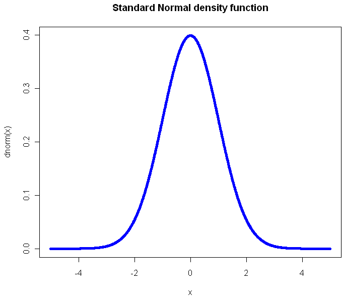
The standard, textbook way to represent a density function looks like this:

Perhaps you have seen this before? (Plot created in R, all source code from this post is included at the end). Not only will you find this plot in statistics books, you’ll also see it in medical texts, sociology, and even economics books. It gives you a clear view of how likely an observation is to fall in a particular range of [latex]x[/latex]. So what’s the problem?

The problem is that what usually concerns us isn’t probability in isolation. What matters is the impact that observations have on some other metric of importance, like the total or average. The key thing we want to know about a distribution is: What range of observations will contribute the most to our expected value, and in what way? We want a measure of influence.

Here’s the plot of the Cauchy density:

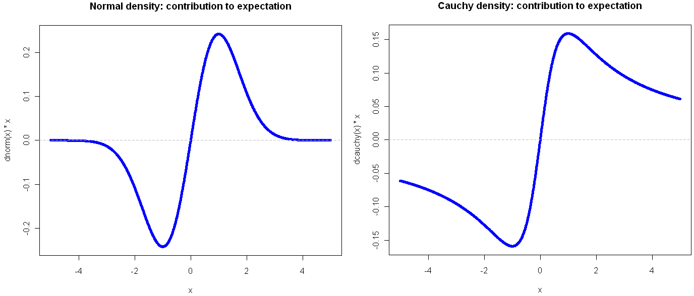
From this view, it doesn’t look all that different from the Normal. Sure it’s a little more narrow, with “fatter tails”, but no radical difference, right? Of course, the Cauchy is radically different from the normal distribution. Those slightly fatter tails give very little visual indication that the Cauchy is so extreme-valued that it has no expected value. Integrating to find the exception gives you infinity in both directions. If your distribution is like this, you’ve got problems and your plot should tell you that right away.

Here’s another way to visualize these two probability distributions:

Go ahead and click on the image above to see the full view. I’ll wait for you…

See? By plotting the density multiplied by the observation value on the y-axis, you get a very clear view of how the different ranges of the function effect the expectation. Looking at these, it should be obvious that the Cauchy is an entirely different beast. In the normal distribution, extreme values are so rare as to be irrelevant. This is why researchers like to find ways to treat their sample as normally distributed: a small sample gives enough information to tell the whole story. But if your life (or livelihood) depends on a sum or total amount, you’re probably best off plotting your (empirical) density in the way shown above.

Another bit of insight from this view is that the greatest contribution to the expectation comes at 1 and -1, which in the case of the Normal isn’t the mean, but rather the second central moment (plus or minus). That’s not a coincidence, but it’s also not always the case, as we shall see. But first, what do things look like when a distribution gets completely out of hand?

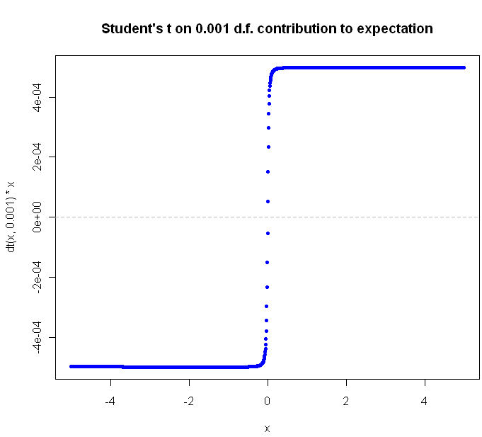
The Student’s t distribution, on 1 Degree of Freedom , is identical to the Cauchy. But why stop at a single DF? You can go all the way down to the smallest (positive) fraction.

The closer you get to zero, the flatter the curve gets. Can we ever flatten it out completely? Not for a continuous distribution with support over an infinite range. Why not? Because in order for the slope of [latex]value * density[/latex] to continue to flatline it indefinitely, the density function would have to be some multiple of [latex]\frac{1}{x}[/latex], and of course the area under this function diverges as we go to infinity, and densities are supposed to integrate to 1, not infinity, right?

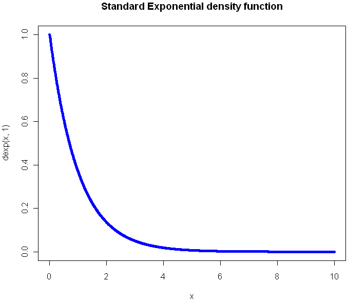
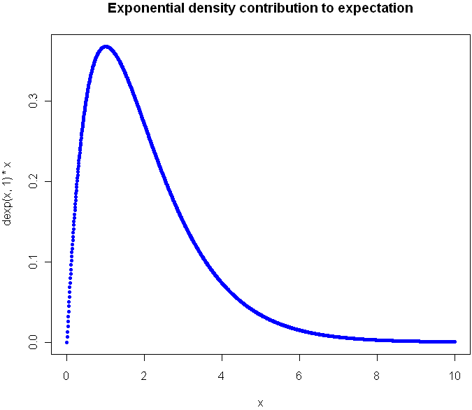
What would the plot look like for a continuous function that extends to infinity in just one direction? Here’s the regular Exponential(1) density function plot:

Now look at the plot showing contribution to expectation:

Were you guessing it would peak at 1?  Again, the expectation plot provides insight into which ranges of the distribution will have the greatest impact on our aggregate values.

Before I go look at an a discrete distribution, try to picture what the expectation curve would look like for the standard [latex]Uniform(0,1)[/latex] distribution. Did you picture a diagonal line?

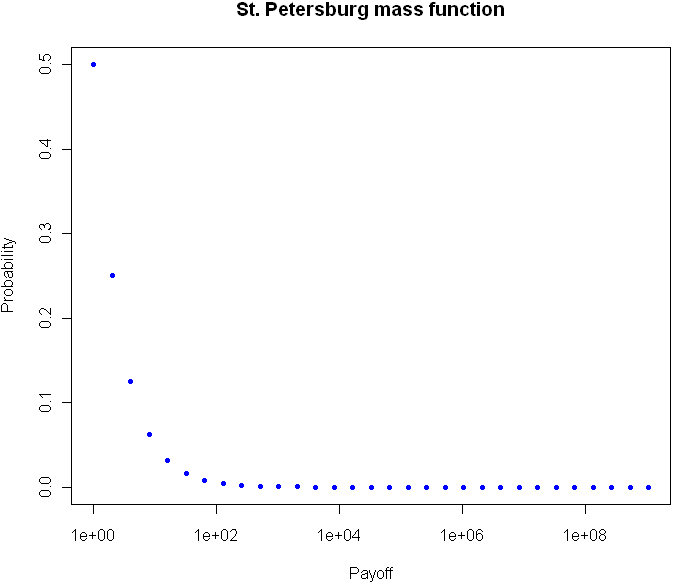
Can we flatten things out completely with an infinitely-supported discrete distribution? Perhaps you’ve heard of the St. Petersburg Paradox. It’s a gambling game that works like this: you flip a coin until tails comes up. If you see one head before a tails, you get $1. For 2 heads you get $2, for 3 heads $4, and so on. The payoff doubles each time, and the chances of reaching the next payoff are halved. The paradox is that even though the vast majority of your winnings will be quite modest, your expectation is infinite.  The regular view of the probability mass function for provides almost no insight:

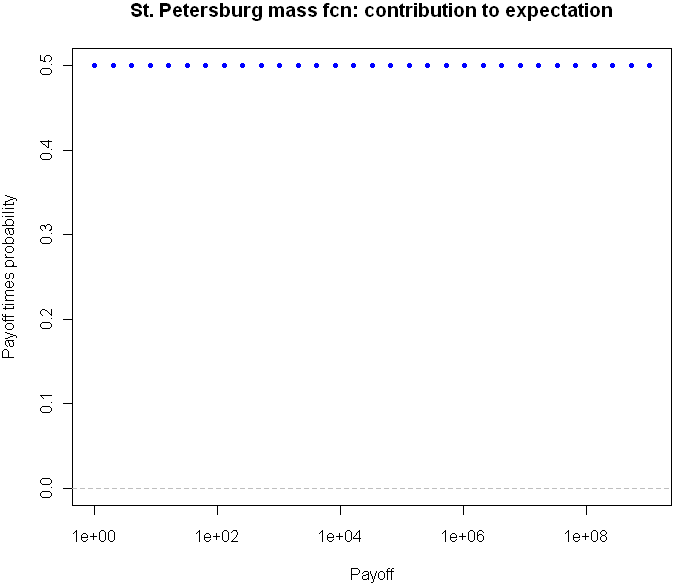
But take a look at the expectation plot:

Flat as a Nebraska wheat field. You can tell right away that something unusual is happening here.

I could go on with more examples, but hopefully you are beginning to see the value in this type of plot. Here is the code, feel free to experiment with other distributions as well.

# Useful way to make dots look like a line
x = seq(-5,5,length=1500)

# You've seen this before. Our good friend the Normal
plot(x,dnorm(x),pch=20,col="blue", main="Standard Normal density function")

# Cauchy looks a little different, but it's not obvious how different it is 
plot(x,dcauchy(x),pch=20,col="blue", main="Cauchy density function")

# New way of plotting the same
plot(x,dnorm(x)*x,pch=20,col="blue", main="Normal density: contribution to expectation")
abline(h=0,lty="dashed",col="gray")

plot(x,dcauchy(x)*x,pch=20,col="blue", main="Cauchy density: contribution to expectation")
abline(h=0,lty="dashed",col="gray")

# Extreme student-t action:
plot(x,dt(x,0.001)*x,pch=20,col="blue", main="Student's t on 0.001 d.f. contribution to expectation")
abline(h=0,lty="dashed",col="gray")


# The Exponential
x = seq(0,10,length=1500)
plot(x,dexp(x,1),pch=20,col="blue", main="Standard Exponential density function")

# The expectation view:
plot(x,dexp(x,1)*x,pch=20,col="blue", main="Exponential mass contribution to expectation")

# What do we see with the St. Petersburg Paradox
x = 2^(0:30)
dStPete <- function(x) {
	return (1/(2*x))
}

# Note the log
plot(x,dStPete(x),pch=20,col="blue", main="St. Petersburg mass function", log="x", xlab="Payoff", ylab="Probability",ylim=c(0,.5))

# Now we see the light
plot(x,dStPete(x)*x,pch=20,col="blue", main="St. Petersburg mass fcn: contribution to expectation", xlab="Payoff", log="x", ylab="Payoff times probability",ylim=c(0,.5))
abline(h=0,lty="dashed",col="gray")

31
May 10

Betting on Pi

I was reading over at math-blog.com about a concept called numeri ritardatari. This sounds a lot like “retarded numbers” in Italian, but apparently “retarded” here is used in the sense of “late” or “behind” and not in the short bus sense. I barely scanned the page, but I think I got the gist of it: You can make money by betting on numbers which are late, ie numbers that haven’t shown up in a while. After all, if the numbers in a lottery or casino are really random, that means it’s highly unlikely that any one number would go a long time without appearing. The “later” the number, the more likely it is to appear. Makes sense, right?

Before plunking down my hard(ly) earned cash at a casino, I decided to test out the theory first with the prototypical random number: Pi. Legend has it that casinos once used digits from Pi to generate their winning numbers. Legend also has it that the digits of Pi are so random that they each appear with almost exactly 1 in 10 frequency. So, given this prior knowledge that people believe Pi to be random, with uniform distribution of digits and no discernible pattern, I can conclude that no one digit should go too long without appearing.

I pulled down the first 10 million digits from here (warning, if you really want this data, right click the link and “save as”). Then I coded up a program in the computer language R to scan through the digits of Pi, one by one, making a series of “fair” bets (1:9 odds) that the next number to appear in the sequence would be the one that had gone longest without appearing. My code is shown below. I had to truncate the data to 1 million digits, and even then this code will take your Cray a good while to process, most likely because I have yet to master the use of R’s faster “apply” functions with complicated loops.

myPi = readLines("pi-10million.txt")[1]

# I think this is how I managed to get Pi into a vector, it wasn't easy.
piVector = unlist(strsplit(myPi,""))
piVector = unlist(lapply(piVector,as.numeric))

# In honor of Goofy Programming Day, I will
# track how long since the last time each digit appeared
# by how many repetitions of that digit are in a vector
ages = c()

# Start us off with nothing in the bank
potHistory = c()

# R just loves long loops like this. Hope you have a fast computer
for(i in 1:1000000) {
	# How did our bet do last round?
	# Skip the first 100 just to build up some data
	if(i > 100) {
		if(betOn == piVector[i]) {
			potHistory = c(potHistory, 9)
		} else {
			potHistory = c(potHistory, -1)
		}
	}

	# Increase all ages by 1 by adding to vector, then set the one we found to 0
	ages = c(ages, 0:9)
	ages = ages[!ages == piVector[i]]

	# Count occurences of each digit, find the top digits by occurence to bet on
	# And you thought Perl was beautiful?
	betOn = as.numeric(names(sort(-table(ages)))[1])
}

# Plot the cumulative sum at 1000 point intervals.
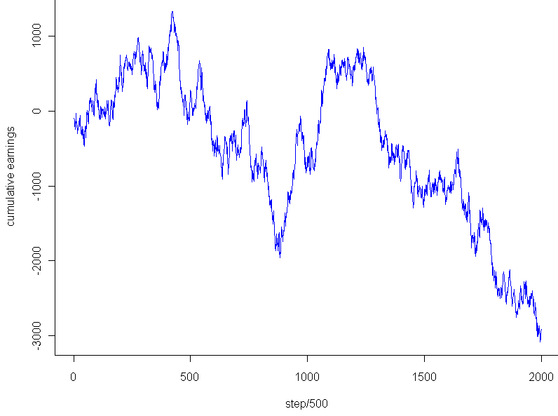
plot.ts(cumsum(potHistory)[seq(0,1000000,500)],pch=20,col="blue",xlab="step/500",ylab="cumulative earnings")

So what was the result? How good was my strategy? After an initial 100 digits to build up data about which digits were latest, I placed a total of 999,900 bets at $1 each. Final earnings: $180. That’s so close to breaking even that it’s almost inconceivable. I had 100,008 wins and 899,892 losses. My winning percentage was 10.0018% percent.

On the face of it, this result seemed almost a little too good, dare I say even suspiciously good, if you know what I mean. How rare is it to get this close (or closer) to the exact perfect proportions after so many trials? Assuming that the number of wins followed a binomial distribution with [latex]p=0.1[/latex], my total wins should follow a Normal distribution with mean 99,990 and variance [latex]n*p*(1-p) = 89,991[/latex] (for an “n” of almost a million and non-minuscule “p”, the Normal approximation to the Binomial should be essentially perfect). Taking the square root of the result, and we get almost exactly 300 as our standard deviation. That’s much larger than the 18 extra wins I had. In fact, the chances that you will land within [latex]18/300 = 0.06[/latex] standard deviations on either side of the Normal’s mean are less than 5%. Before getting too worked up over this result, I decided to take a look at the graph. Using the code:

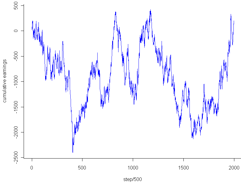
plot.ts(cumsum(potHistory)[seq(0,1000000,500)],pch=20,col="blue",xlab="step/500",ylab="cumulative earnings")

I got this:

The graph looks pretty much like any random walk, doesn’t it? So the fact that I ended up breaking almost exactly even had to do with the stopping point, not any “unusual” regularity. Just to see if I might salvage any mystery, I tested the very lowest point, -$2,453, which occurred after 202,133 trails. Even that falls within 2 standard deviations of the expected mean for that number of trials, and of course cherry picking the most extreme point to stop at isn’t a fair way to go about this. Any last hope that the graph might be unusual? I plotted a couple random walks using numbers generated in R. Most of them looked like this:

This looks to have the same level of “jaggedness” as  the results of my bet on Pi. Unfortunately, I am forced to conclude that the promising strategy of “late number” gambling turned out to be fairly retarded after all, at least so far as it applies to the digits of Pi.


29
May 10

Weekend art in R (part 1?)


As usual click on the image for a full-size version. Code:

par(bg="black")
par(mar=c(0,0,0,0))
plot(c(0,1),c(0,1),col="white",pch=".",xlim=c(0,1),ylim=c(0,1))
iters = 500
for(i in 1:iters) {
	center = runif(2)
	size = rbeta(2,1,50)

	# Let's create random HTML-style colors
	color = sample(c(0:9,"A","B","C","D","E","F"),12,replace=T)
	fill = paste("#", paste(color[1:6],collapse=""),sep="")
	brdr = paste("#", paste(color[7:12],collapse=""),sep="")

	rect(center[1]-size[1], center[2]-size[2], center[1]+size[1], center[2]+size[2], col=fill, border=brdr, density=NA, lwd=1.5)
}