probability


21
May 11

Problematic quote of the day

“Ellsberg offered several groups of people a chance to bet on drawing either a red ball or a black ball from two different urns, each holding 100 balls. Urn 1 held 50 balls of each color; the breakdown in Urn 2 was unknown. Probability theory would suggest that Urn 2 was split 50-50, for there was no basis for any other distribution.”

From page 280 of Against the Gods: The Remarkable Story of Risk.


5
Nov 10

Livin’ la Vida Poisson

Yes, I did just mix English, Spanish and French. And no, I am not living the “fishy” life, popular opinion to the contrary. Here’s the story. As someone who spends the majority of his time working online, with no oversight, I notice that I tend to drift a lot. I don’t play solitaire, or farm for virtual carrots, but I do wander over to Reddit more than I should, or poke around in this or that market in virtual assets to see if anything interesting has shown up. To some extent this can be justified. Many, perhaps all, of my profitable ventures have come from keeping my eyes open, poking around, doing my best to understand the digital world. On the other hand, at times I feel like I’ve been drifting aimlessly, that I’m all drift and no focus. My existing projects are gathering dust while I chase after shiny new things.

That’s the feeling, anyway. What does the evidence say? To keep track of what I was really doing, and perhaps nudge me towards more focus, I set a stopwatch to go off every 15 minutes. When it did, I would stop, write down what I was doing at that moment, and continue on. Perhaps you can see how these set intervals might provide an incentive to, shall we say, cheat? Especially right after the stopwatch chimed, I knew that whatever I did for the next few minutes was “free”, untracked. So I decided that I would have to write down everything I did during those 15 minute intervals, which worked sometimes, othertimes not so well.

My current solution? Setup a bell which chimes at random intervals, with an average time between chimes of 15 minutes. To hear what the bell sounds like, Go ahead and try it out, I think you’ll find it makes a nice sound. Leave that page open while you read the rest of this post, see how many times it rings.

At any rate, in order to randomize how long the wait was between chimes, I used a little something called a Poisson process. Actually, what I used was the Binomial approximation to the Poisson built from multiple Bernoulli trials, which results in wait times that are Exponential. Wait! Did you get all that? If so, then skip ahead until things look interesting. Otherwise, here’s more detail about how this works:

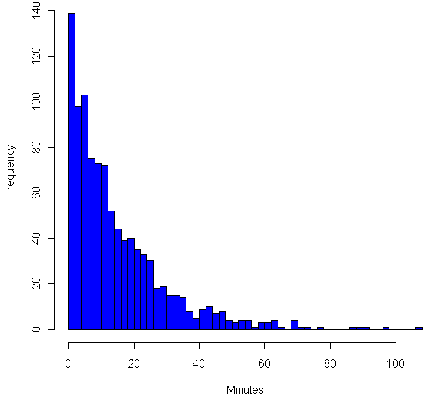
In order to determine the length of time between chimes, my computer generates a random number number between 0 and 1. If this random number is less than 1/15, then the next chime is in just one minute. Otherwise, the computer generates another random number and adds one minute to the time between chimes. On average, it will take 15 tries to get a number below 1/15, so the average time between chimes will be 15 minutes. However, to call 15 minutes the average is somewhat misleading. Here are the frequencies of different wait times (source code in R at the end):


As you can see, the most common time between chimes is just one minute. Strange, no? What’s going on here is that each test to see if the random number is below 1/15 is a Bernoulli trial, which is basically Italian for “maybe it succeeds, maybe it fails”. In this case “success” has probability of 1/15, failure happens the other 14 out of 15 times. In cases where probability is small, and you end of doing a lot of trials, the total number of successes over a given time period will have the Poisson distribution. The “Poisson” here is a Frenchman, who may or may not have smelled like his surname, but who certainly understood The Calculus as well as anyone in the early 1800’s. To get an even better approximation of the Poisson, I could have used trails with probability of success of 1/900, then treated each failure as another second of waiting time. That would have made the graph above smoother.

But wait! I didn’t show you a graph of the Poisson. I showed you a graph of something that approximates the exponential distribution. The number of chimes per hour is (roughly) Poisson distributed, but the waiting time between each chime is exponential, which means shorter wait times are more frequent, but no length of time, no matter how long, can be ruled out. In fact, the exponential distribution is the only (continuous) distribution which is “memoryless”. If you have waited 15 minutes for a chime, your expected wait time is still…. 15 minutes. In fact, your expected wait is independent of how long you have waited so far. The exponential distribution is a “maximal entropy” distribution, entropy in this case is related to how much you know. With the exponential, no matter how long you’ve waited, you still don’t know anything more than when you started waiting.

If you’ve been tuning out and scanning this post, now would be a good time to tune back in. I promise new and interesting things ahead!

It’s one things to understand the memoryless property of the exponential, even down to the mathematical nitty-gritty. It’s quite another to actually live with the exponential. No matter how well I know the formulas, I can’t shake the felling that the longer I have waited in between bell rings, the sooner the next chime must be coming. Certainly, it should be due any time now! While I “know” that any given minute has exactly the same probably as the next to bring with it the bell, the longer I wait, the nearer I feel the the next chime must be. After all, the back of my mind insists, once the page loads the wait time has been set into stone. However it was distributed before, it’s now a constant. Every minute you wait you are getting closer to the next bell, whenever it might have been set to come. I keep wanting to know more than I did a minute ago about about when the next bell will arrive.

This isn’t the only way in which I find my psyche battling with my intellect. I would also swear that over time the distribution of short waits and long waits evens out. Now, by the law of large numbers, it’s true that the more chimes I sit through, the closer the mean wait time will approach 15 minutes. However, even if you’ve just heard three quick bells in a row, that has absolutely no bearing on how long the wait will be between the next three chimes. The expected wait times going forward are completely independent of the wait times in the past. The mean remains 15 minutes, the median remains 10.4 minutes. Yet that’s not what I feel is happening, and over the past two weeks of experimenting with this I would swear that on days when there are a number of unusually quick intervals, these have been followed, later that very the same day, with unusually long intervals. And vice versa. It feels like things are evening out.

It’s possible that when my computer wakes up from a sleep mode, my web browser doesn’t remember where it was in a countdown to refreshing the chime page. So I reload it. Now, in theory, if you “reload” an exponential wait time while in process, this has absolutely no effect on your eventual wait time until the next chime. Yet anytime I reload the page, I have a moment of doubt as to whether I’m “cheating” in some way, to make what would have been a long wait shorter. In this case, the back of my mind says the exact opposite of its previous bias: because I am reloading a page that has been waiting a long time, this means that the wait time would have been really long. By starting the process anew, I’m increasing the chances of a short chime time.

Before you call me a nut, try living for a while with the timer running the background. Keep track of what you are doing if you want (and BTW I’ve found this to be every enlightening and more than a little sad), but mostly keep track of how you feel about the timing. Try reloading the page if you don’t hear a chime for a while. How does that feel? I suspect that in some ways humans were very well hard wired to understand probabilities. Yet I also suspect our wiring hinders how we understand probability, a suspicion backed up by all those gamblers out there waiting for the lucky break that’s well overdue.

CODE:

iters = 1000
results = rep(0,iters)
for (i in 1:iters) {
	minutes = 1
	while(runif(1)>(1/15)){
		minutes = minutes + 1
	}
	
	results[i] = minutes
}

hist(results, breaks=40, col="blue", xlab="Minutes")

30
Aug 10

The Chosen One

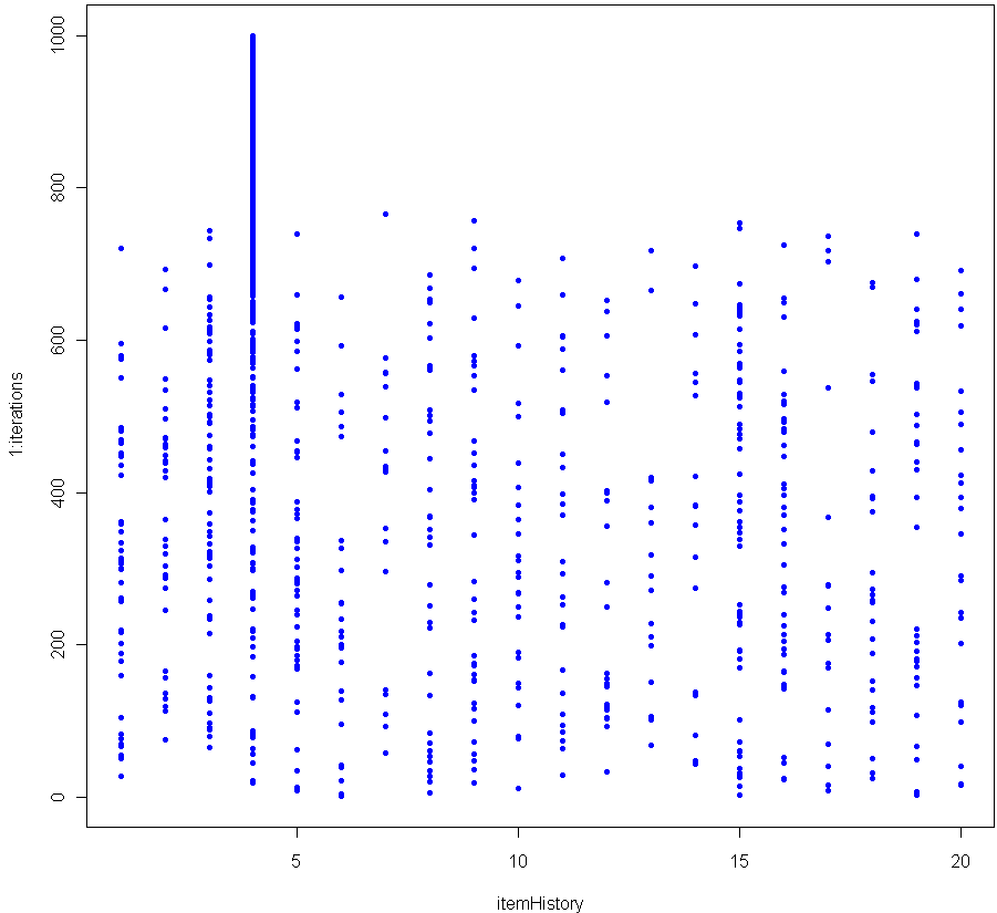
Toss one hundred different balls into your basket. Shuffle them up and select one with equal probability amongst the balls. That ball you just selected, it’s special. Before you put it back, increase its weight by 1/100th. Then put it back, mix up the balls and pick again. If you do this enough, at some point there will be a consistent winner which begins to stand out.

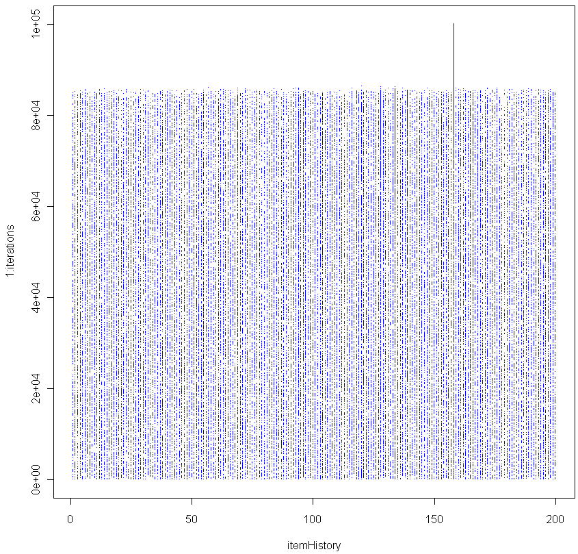
The graph above shows the results of 1000 iterations with 20 balls (each victory increases the weight of the winner by 5%). The more balls you have, the longer it takes before a clear winner appears. Here’s the graph for 200 balls (0.5% weight boost for each victory).

As you can see, in this simulation it took about 85,000 iterations before a clear winner appeared.

I contend that as the number of iterations grows, the probability of seeing a Chosen One approaches unity, no matter how many balls you use. In other words, for any number of balls, a single one of them will eventually see its relative weight, compared to the others, diverge. Can you prove this is true?

BTW this is a good Monte Carlo simulation of the Matthew Effect (no relation).

Here is the code in R to replicate:

numbItems = 200
items = 1:numbItems
itemWeights = rep(1/numbItems,numbItems) # Start out uniform
iterations = 100000
itemHistory = rep(0,iterations)

for(i in 1:iterations) {
	chosen = sample(items, 1, prob=itemWeights)
	itemWeights[chosen] = itemWeights[chosen] + (itemWeights[chosen] * (1/numbItems))
	itemWeights = itemWeights / sum(itemWeights) # re-Normalze
	itemHistory[i] = chosen
}

plot(itemHistory, 1:iterations, pch=".", col="blue")

After many trials using a fixed large number of balls and iterations, I found that the moment of divergence was amazingly consistent. Do you get the same results?


8
Aug 10

Seeing angels in the architecture

Sorry for the long delay between posts; I was temporarily sucked in to the infinite. While doing some reading about set theory (foundational stuff for probability and, in fact, all of mathematics), I veered off into the infinite and had a hard time climbing back out. I’m guessing you already know most of the basics about sets: compliments and unions and intersections. You may even know some of the stranger parts, like G. Cantor’s cascading crescendo of cardinalities. But knowing those in a cursory way (and really, that’s all a work-a-day statistician or even probabilist needs) isn’t the same as really exploring them.

Looking up again now after several weeks, I feel like I’ve traveled three levels deep in a dream, lost in a purgatory I could only escape by answering questions like  “Is a line made up of points, or does it have points?”, “Is it possible to count what you cannot fully name”, and “In an unbounded universe, is the compliment of the compliment of an object the same as the original object?”. I know, I know. I should have taken that left back at Albuquerque, I shouldn’t have swallowed the red pill. Still, it’s been an interesting trip to say the least, and I feel like I may now be coming back up the the surface, a little bit wiser and a lot more confused than when I began.

Meanwhile, I’ve added a couple items to the “Manifesto” and, The Architect permitting, will be posting a theory on Types of Randomness soon. Post should take between 1 and 10 days to complete, with 95% confidence. Hum… better make that an 80% confidence interval, I still haven’t wrapped my head around the whole idea of forcing.


19
Jul 10

R: Clash of the cannon cycles

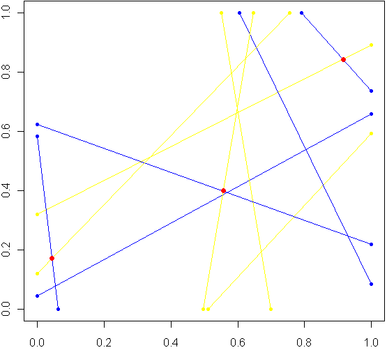
Imagine a unit square. Every side has length 1, perfectly square. Now imagine this square was really a fence, and you picked two spots at random along the fence, with uniform probability over the length of the fence. At each of these two locations, set down a special kind of cannon. Just like the light cycles from Tron, these cannons leave trails of color. To aim each cannon, pick another random point from one of the three other sides of the fence, and aim for that point.

Sometimes there will be a collision within the square, other times no. The image at top shows the results of five trials. The red dots are where the trails from a pair of cannons collided. My burning question: What is the distribution for these dots? Before reading on, try to make a guess. Where will collisions be most likely to happen?

Somewhere in the world, there lives a probabilist who could come up with a formula for the exact distribution in an hour, but that person doesn’t live in my house, so I took the Monte Carlo approach, coded in R:

# Functions to pick two points, not on the same side:
m2pt <- function(m) {
	if(m <1) {
		myPoint = c(5,m,0)
	} else if (m < 2) {
		myPoint = c(6,1,m %% 1) 
	} else if (m < 3) {
		myPoint = c(7,1-(m %% 1),1)
	} else {
		myPoint = c(8,0,1-(m %% 1))
	}
	return(myPoint)
}		

get2pts <- function() {
	pt1 = m2pt(runif(1,0,4))
	pt2 = m2pt(runif(1,0,4))
	
	# Make sure not both on the same sides. If so, keep trying
	while(pt1[1] == pt2[1]) {
		pt2 = m2pt(runif(1,0,4))
	}
	return(c(pt1[2:3],pt2[2:3]))
}

# Optional plot of every cannon fire line. Not a good idea for "iters" more than 100
#windows()
#plot(0,0,xlim=c(0,1),ylim=c(0,1),col="white")		
		
# How many times to run the experiment
iters = 10000

# Track where the intersections occur
interx = c()
intery = c()

for(i in 1:iters) {
	can1 = get2pts()
	can2 = get2pts()
	
	# Optional plot of every cannon fire line. Not a good idea for "iters" more than 100 
	#points(c(can1[1],can1[3]),c(can1[2],can1[4]),pch=20,col="yellow")
	#segments(can1[1],can1[2],can1[3],can1[4],pch=20,col="yellow",lwd=1.5)
	#points(c(can2[1],can2[3]),c(can2[2],can2[4]),pch=20,col="blue")
	#segments(can2[1],can2[2],can2[3],can2[4],pch=20,col="blue",lwd=1.5)

	# See if there is a point of intersection, find it. 
	toSolve = matrix(c( can1[3]-can1[1], can2[3]-can2[1], can1[4]-can1[2], can2[4]-can2[2]),byrow=T,ncol=2)
	paras = solve(toSolve, c( can2[1]-can1[1], can2[2]-can1[2]))
	
	solution = c(can1[1] + paras[1]*(can1[3]-can1[1]), can1[2] + paras[1]*(can1[4]-can1[2]))
	
	# Was the collision in the square
	if(min(solution) > 0 && max(solution) < 1) {
		# Optional plot of red dots
		# points(solution[1],solution[2],pch=20,col="red",cex=1.5)
		
		# if this intersection is in square, plot it, add it to list of intersections
		interx = c(interx, solution[1])
		intery = c(intery, solution[2])
	}
}

windows()
plot(interx, intery, pch=20,col="blue",xlim=c(0,1),ylim=c(0,1))

After carefully writing and debugging much more code than I expected, I ran a trial with several thousand cannon fires and plotted just the collisions. Here is what I saw:

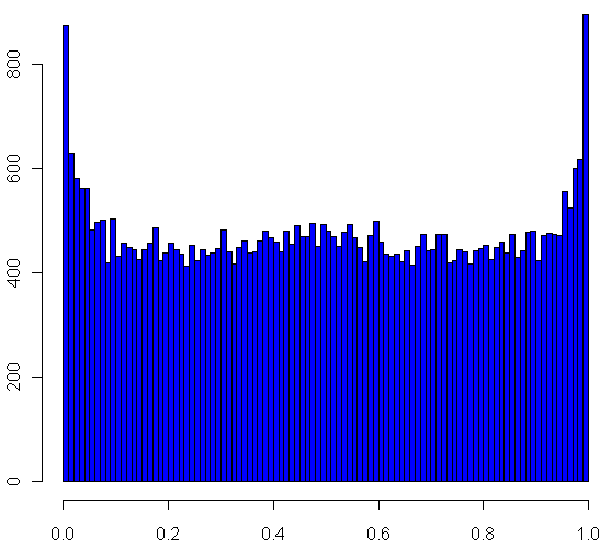
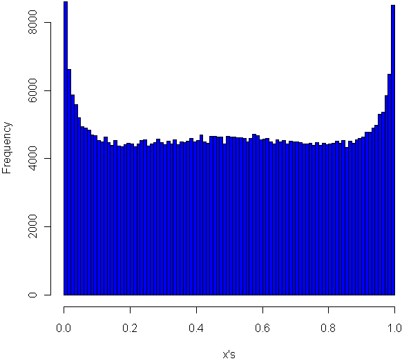
Looks pretty uniform, doesn't it? If it is, I will have gone a very long way just to replicate the bi-variate uniform distribution. My own original guess was that most collisions, if they happened in the square, would be towards the middle. Clearly this wasn't the case. Looks can be deceiving, though, so I checked a histogram of the x's (no need to check the y's, by symmetry they have the same distribution):

Very interesting, no? The area near the edges appears more likely to have a collision, with an overall rounded bowl shape to the curve. The great thing about Monte Carlo simulations is that if something unexpected happens, you can always run it again with more trials. Here I changed "iters" to 100,000, ran the code again, and plotted the histogram.

hist(interx, breaks=100, col="blue",xlab="x",main="Histogram of the x's")

Now its clear that the distribution spikes way up near the edges, and appears to be essentially flat for most of the middle area. It seems like it may even go up slightly at the very middle. Just to be sure, I ran a trial with one million iterations:

Now it definitely looks like a small upward bulge in the middle, though to be sure I would have to do run some statistical tests or use an even larger Monte Carlo sample, and given how inefficient my code is, that could take the better part of a week to run. So for today I'll leave it at that.

One final statistic of note: During my run of one million iterations, 47.22% of all collisions happened inside the box. What do you think, is the true, theoretical ratio of collisions within the box a rational number?


10
Jul 10

Photo without caption


9
Jul 10

100 Prisoners, 100 lines of code

In math and economics, there is a long, proud history of placing imaginary prisoners into nasty, complicated scenarios. We have, of course, the classic Prisoner’s Dilemma, as well as 100 prisoners and a light bulb. Add to that list the focus of this post, 100 prisoners and 100 boxes.

In this game, the warden places 100 numbers in 100 boxes, at random with equal probability that any number will be in any box. Each convict is assigned a number. One by one they enter the room with the boxes, and try to find their corresponding number. They can open up to 50 different boxes. Once they either find their number or fail, they move on to a different room and all of the boxes are returned to exactly how they were before the prisoner entered the room.

The prisoners can communicate with each other before the game begins, but as soon as it starts they have no way to signal to each other. The warden is requiring that all 100 prisoners find their numbers, otherwise she will force them to listen to hundreds of hours of non-stop, loud rock musician interviews. Can they avoid this fate?

The first thing you might notice is that if every prisoner opens 50 boxes at random, they will have a [latex]0.5[/latex] probability of finding their number. The chances that all of them will find their number is [latex](\frac{1}2)^{100}[/latex], which is approximately as rare as finding a friendly alien with small eyes. Can they do better?

Of course they can. Otherwise I wouldn’t be asking the question, right? Before I explain how, and go into a Monte Carlo simulation in R, you might want to think about how they can do it. No Googling!

All set? Did you find a better way? The trick should be clear from the code below, but if not skip on to the explanation.

# How many times should we run this experiment?
iters = 1000
results = rep(0,iters)

for(i in 1:iters) {
	# A random permutation:
	boxes = sample(1:100,100)

	# Labels for our prisoners
	prisoners = 1:100

	# Track how many "winners" we have
	foundIt = 0

	# Main loop over the prisoners
	for(prisoner in prisoners) {

		# Track the prisoners path
		path = c(prisoner)

		tries = 1

		# Look first in the box that matches your own number
		inBox = boxes[prisoner]

		while(tries < 50) { 			 			path = c(path, inBox) 			 			if(inBox == prisoner) { 				#cat("Prisoner", prisoner, "found her number on try", tries, "\n") 				foundIt = foundIt + 1 				break; 			} else { 				# Follow that number to the next box 				inBox = boxes[inBox] 			} 			tries = tries+1 		} 		 		# cat("Prisoner", prisoner, "took path", paste(path, collapse=" -> "), "\n")
	}

	# How many prisoners found their numbers?
	cat("A total of", foundIt, "prisoners found their numbers.\n")
	flush.console()
	results[i] = foundIt
}

hist(results, breaks=100, col="blue")

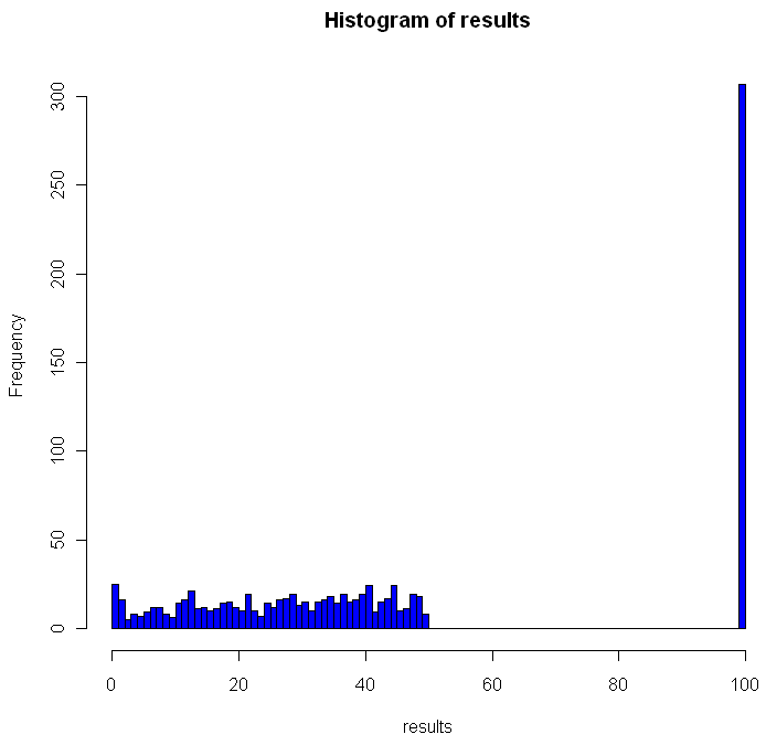
Here is what one of my plots looked like after running the code:

Out of the 1000 times I ran the experiment, on 307 occasions every single prisoner found his number. The theoretical success rate is about 31%. So, if it’s not clear from the code, what was the strategy employed by the prisoners and how does it work?

One way to look at the distribution of numbers in boxes is to see it as a permutation of the numbers from 1 to 100. Each permutation can be partitioned into what are called cycles. A cycle works like this: pick any number in your permutation. Let’s say it’s 23. Then you look at the number the 23rd place (ie the number in the 23rd box, counting from the left). If that number is 16, you look at the number in the 16th place. If that number is 87, go open box number 87 and follow that number. Eventually, the box you open up will have the number that brings you back to where you started, completing the cycle. Different permutations have different cycles.

The key for the prisoner is that by starting with the box that is the same place from the left as his number, and by following the numbers in the boxes, the prisoner guarantees that if he is in a cycle of length less than 50, he will eventually open the box with his number in it, which would complete the cycle he began. One way to envision cycles of different lengths is to think about the extreme cases. If a particular permutation shifted every single number over one to the left (and wrapped number 1 onto the end), you would have a single cycle of length 100. Box 1 would contain number 2, box 2 number 3 and so on. On the other hand, if a permutation flipped every pair of consecutive numbers, you would have 50 cycles, each of length 2: box 1 would have number 2, box 2 would have number 1. Of course if your permutation doesn’t change anything you have 100 cycles of length 1.

As you can see from the histogram, when using this strategy you can never have between 50 and 100 winning prisoners. Anytime you have a single cycle of length greater than 50, for example 55, then all 55 prisoners who start on that cycle will fail to find their number. If no cycles are longer than 50, everyone wins. Just how rare are different cycles of different lengths? For the math behind that check out this excellent explanation by Peter Taylor of Queen’s University.

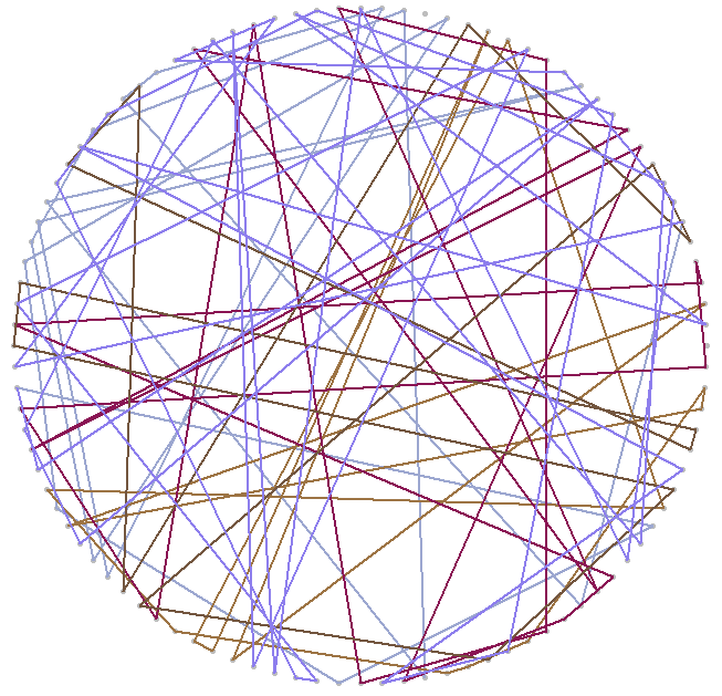
Before moving on I wanted to visualize these cycles. Try running the code below:

# Unit circle
plot(0,0,xlim=c(-1,1),ylim=c(-1,1),col="white",ann=FALSE, xaxt="n", yaxt="n")
for(i in 1:100) {
	points(cos(2*i/100*pi), sin(2*i/100*pi),pch=20,col="gray")
}

mySample = sample(1:100,100)
for(i in 1:100) {
	found = FALSE
	nextItem = i

	# Pick a random color for this cycle
	color = sample(c(0:9,"A","B","C","D","E","F"),12,replace=T)
	lineColor = paste("#", paste(color[1:6],collapse=""),sep="")

	while(!found) {
		# Draw the cycle

		segments(cos(nextItem/50*pi), sin(nextItem/50*pi), cos(mySample[nextItem]/50*pi), sin(mySample[nextItem]/50*pi),col=lineColor,lwd=2)
		Sys.sleep(.4)
		if(mySample[nextItem] == i) {
			found = TRUE
		} else {
			nextItem = mySample[nextItem]
		}
	}
}

You can adjust the “Sys.sleep()” parameter to make the animation faster. I recommend running the code to see how the cycles “develop” over time, but here’s a snapshot of what I got:


2
Jul 10

Word games in probability and R

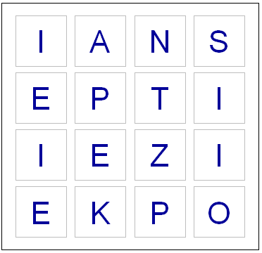
Last night, while playing Boggle, we ended up with a board without a single vowel. Not even a “Y” or “Qu”. This seemed fairly unusual, so I wondered what the chances were of such an occurrence. I found an online list of the letters each die has, and I could have written down the number of vowels on each one by hand, but whenever possible I like to do things by computer. So I fired up Hal and asked for some help with the calculations.

Apparently some European boards use a 5 x 5 grid, but here in the land of the Maple leaf our board has 16 cubes. Here are the letters on them, as I coded them into R:

d1 = c('S','R','E','L','A','C')
d2 = c('D','P','A','C','E','M')
d3 = c('Qu','B','A','O','J','M')
d4 = c('D','U','T','O','K','N')
d5 = c('O','M','H ','R','S','A')
d6 = c('E','I','F','E','H','Y')
d7 = c('B','R','I','F','O','X')
d8 = c('R','L','U','W','I','G')
d9 = c('N','S','O','W','E','D')
d10 = c('Y ','L','I','B','A','T')
d11 = c('T','N','I','G','E','V')
d12 = c('T','A','C','I','T','O')
d13 = c('P','S','U','T','E','L')
d14 = c('E','P','I','S','H ','N')
d15 = c('Y','K','U','L','E','G')
d16 = c('N','Z','E','V','A','D')

So now I had to check how many vowels were on each die. Here’s the code I used for this:

vowels = c('A','E','I','O','U','Qu','y')
vowelsFound = rep(0,16)
for(i in 1:16) {
	found = 0
	die = eval(parse(text=paste("d",i,collapse="",sep="")))
	for(l in die) {
		# Check to see if this letter is in the vowels vector
		if(l %in% vowels) {
			found = found + 1
		}
	}
	vowelsFound[i] = found
}

# Probabilities of getting a vowel for each die
pVowels = vowelsFound/6

# Probability of getting no vowel for each die
pNoVowels = 1 - pVowels

# Chance that we will get not a single vowel, including "y" and "Qu"
print(prod(pNoVowels))

If you run the code above, you should see that the probability of getting no vowels (including “Y” and “Qu”) is 0.000642. That works out to one in every 1557 boards. So it’s quite rare, but by no means so extraordinary that it crosses the Universal probability bound. Also, it’s not enough to just calculate how rare your event is, or how rare any similar or more extreme event is, and then be astounded. You also have to include all the other possible events that would have left you amazed. What about getting all vowels (much more rare)? What about getting 8 or 9 E’s, or a row or column of all A’s or E’s? It’s likely that if you add up all probabilities of all the rare events which might leave you amazed, you’ll end up with a good chance of amazement every time.

I could have stopped here, but having coded the dice, I decided to create a simplified version of the game in R. If I have a chance over the next few days I’ll add some more features.

# You will need to download a dictionary file. I found one here:
# http://svn.pietdepsi.com/repos/projects/zyzzyva/trunk/data/words/north-american/owl2-lwl.txt
words = read.table("wordlistData.dat", colClasses = "character")
words = unlist(words[,1])

# Create a random board. Plot it.
board = diag(4)
dice = sample(1:16,16)
cntr = 4
for(i in dice) {
	die = eval(parse(text=paste("d",i,collapse="",sep="")))
	board[floor(cntr/4), (cntr %% 4) + 1] = sample(die,1)
	cntr = cntr + 1
}

plot(0,0,xlim=c(0,4),ylim=c(0,4),col="white",ann=FALSE, xaxt="n", yaxt="n" )

for(m in 1:4) {
	for(n in 1:4) {
		text(m-.5,n-.5,labels=board[m,n],cex=2.75,col="#000099")
		# Draw a square the easy way
		points(m-.5,n-.5,pch=0,cex=10,lwd=1.5,col="gray")
	}
}

# How many seconds to give for each round
gameTime = 180

START_TIME = proc.time()[3]	
elapsed = 0

# Simple scoring, with 1 point per letter. 
# Dictionary only has words length 3 or longer
score = 0

cat("Find words. Hit enter after each word.\n")
while(elapsed < gameTime) {
	myWord = scan(n=1, what=character()) # Get a single word
	elapsed = signif(proc.time()[3] - START_TIME, digits=4)
	if (length(myWord)==0) {
		cat("You have", gameTime - elapsed, "seconds left. Keep going!\n")
	} else {
		
		if(elapsed < gameTime) {
			# Check if it's a real word, see if it is in dictionary
			# Convert their guess to uppercase letter
			myWord = toupper(myWord)
			
			# If it is in the dictionary, give them points
			if(myWord %in% words) {
				# Make sure they haven't used this word before TODO
			
				# Add it to their score
				score = score + nchar(myWord)
				cat("Congratulations. You are up to", score, "points.")
				cat("You have", gameTime - elapsed, "seconds left. Keep going!\n")
			} else {
				# If it isn't in the dictionary, let the user know that they got it wrong.
				cat("Sorry, that is not in the dictionary. Keep trying!\n")
			}
			
			
		}
	}
} 

cat("Out of time! ")
cat("Your final score was:", score, "points.")

Enjoy the game. Let me know if you notice any issues or have suggestions!


18
Jun 10

Those dice aren’t loaded, they’re just strange

I must confess to feeling an almost obsessive fascination with intransitive games, dice, and other artifacts. The most famous intransitive game is rock, scissors, paper. Rock beats scissors.  Scissors beats paper. Paper beats rock. Everyone older than 7 seems to know this, but very few people are aware that dice can exhibit this same behavior, at least in terms of expectation. Die A can beat die B more than half the time, die B can beat die C more than half the time, and die C can beat die A more than half the time.

How is this possible? Consider the following three dice, each with three sides (For the sake of most of this post and in my source code I pretend to have a 3-sided die. If you prefer the regular 6-sided ones, just double up every number. It makes no difference to the probabilities or outcomes.):

Die A: 1, 5, 9
Die B: 3, 4, 8
Die C: 2, 6, 7

Die A beats B [latex]5/9[/latex] of the time which beats C [latex]5/9[/latex] of the time which beats A [latex]5/9[/latex] of the time. Note that the ratios don’t all have to be the same. Here’s another intransitive trio:

Die A: 2, 4 ,9
Die B: 1, 8, 7
Die C: 3, 5, 6

Take a moment to calculate the relative winning percentages, or just trust me that they are not all the same…. Did you trust me? Will you trust me now in the future?

In order to find these particular dice I wrote some code in R to automate the search. The following functions calculate the winning percentage for one die over another and check for intransitivity:

# Return the proportion of the time that d1 beats d2. 
# Dice need to have same number of sides
calcWinP <- function(d1,d2) {
	sides = length(d1)
	d1Vd2 = 0
	
	for(i in 1:sides) {
		for(j in 1:sides) {
			if(d1[i] > d2[j]) {
				d1Vd2 = d1Vd2 + 1
			}
		}
	}
	
	return( d1Vd2/(sides^2) )
}

# Assumes dice have no ties. 
# All dice must have the same number of sides.
# How many times do I have to tell you that?
checkIntransitivity <- function(d1,d2,d3) {
	d1beatsd2 = calcWinP(d1,d2)
	
	if (d1beatsd2 > 0.5) {
		if(calcWinP(d2,d3) > 0.5) {
			if(calcWinP(d3,d1) > 0.5) {
				return(TRUE)
			}
		}
	} else {
		# Check if d1 beats d3, if so check if d3 beats d2
		if(calcWinP(d1,d3) > 0.5) {
			if(calcWinP(d3,d2) > 0.5) {
				return(TRUE)
			}
		}
	}
	# Regular old transitivity.
	return(FALSE)
}

I then checked every possible combination. How many unique configurations are there? Every die has three numbers on it, and you have three die for a total of nine numbers. To make things simpler and avoid ties, no number can be used more than once. If each sides of a die was ordered and each of the die was ordered, you’d have [latex]9![/latex] different combinations, which is to say a whole mess of them. But our basic unit of interest here isn’t the digits, it’s the dice. So let’s think about it like this: For die A you can choose 6 of the 9 numbers, for die B you can pick 3 of the remaining 6, and for die C you’re stuck with whatever 3 are left. Multiply this all together:

choose(9,6)*choose(6,3)

and you get 1680 possibilities. But wait? What’s that you say? You don’t care which die is A, which is B, and which is C? Fantastic. That reduces the number of “unique” configurations by [latex]3![/latex], which is to say 6, at least if my back-of-the-envelope calculations are correct. Final tally? 280.

Not bad. Unfortunately, there no obvious way to ennumerate each of these 280 combinations (at least not to me there isn’t). So I ended up using a lot of scratch work and messing around in the R console until I had what I believed to be the right batch. Sorry, I no longer have the code to show you for that. After testing those 280 configurations, I found a total of 5 intransitive ones, including the 2 dice shown previously and the following 3 sets:

Die A: 2, 9, 3
Die B: 1, 6, 8
Die C: 4, 7, 5

Die A: 7, 1, 8
Die B: 5, 6, 4
Die C: 9, 3, 2

Die A: 7, 3, 5
Die B: 2, 9, 4
Die C: 8, 6, 1

Did I make a mistake? According to my calculations, [latex]5/280[/latex] of the combinations are intransitive. That represents 1.786% of the total. How might I very this? That’s right, it’s Monte Carlo time.

Using the following code, I created all [latex]9![/latex] permutations of dice and sides, then sampled from those 362,880 sets of dice many, many times:

library(e1071) # Makes making permutations easy
allPerms = permutations(9)
intransFound = 0
for(i in 1:dim(allPerms)[1]) {
	d1 = allPerms[i,1:3]
	d2 = allPerms[i,4:6]
	d3 = allPerms[i,7:9]
	if(checkIntransitivity(d1,d2,d3)) {
		intransFound = intransFound + 1
	}
}

print(intransFound)
	
found = 0	
tries = 100000
for(i in 1:tries) {
	one2nine = sample(1:9,9)
	d1 = one2nine[1:3]
	d2 = one2nine[4:6]
	d3 = one2nine[7:9]
	
	if( checkIntransitivity(d1,d2,d3)) {
		found = found + 1
		# Uncomment below if you want to see them.
		#print("found one")
		#print(d1)
		#print(d2)
		#print(d3)
		#flush.console()
	}
}

print(found/tries)

Final percentage: 1.807%. That’s pretty close to [latex]5/280[/latex], and much closer than it is to either [latex]4/280[/latex] or [latex]6/280[/latex], so I’m going to conclude that I got them all and got it right.

What happens if your dice have fewer, or more, sides? Turns out you need at least 3 sides to achieve intransitivity. Can you have it with 4 sides? What about 5, 6, or 7? To estimate the fraction of dice configurations which are intransitive for different numbers of sides I wrote the following code. Note that this could take a while to run, depending on the number of “tires” you use:

# Transitivity vs sides.
results = rep(0,6)
tries = 100000
	
for(j in 4:12) {
	found = 0	

	for(i in 1:tries) {
		one2nine = sample(1:(3*j),(3*j))
		d1 = one2nine[1:j]
		d2 = one2nine[(j+1):(2*j)]
		d3 = one2nine[(2*j+1):(3*j)]
		
		if( checkIntransitivity(d1,d2,d3)) {
			found = found + 1
		}
	}
	
	results[j] = found/tries
	print("Found:")
	print(results[j])
	flush.console()
}

If you wait through all that you might notice some interesting patters emerge, which probably have explanations rooted in theory but it’s getting on nap time, so I’ll wrap this post up.

I think what fascinates me the most about intransitive dice, and games like rock, scissors, paper, is that they represent breakdowns in what math folks like to call a “total order”. Most of our calculations are done in this nice land of numbers where you can count on transitivity. [latex]A>B[/latex] and [latex]B>C[/latex], therefore [latex]A>C[/latex]. Every item has it’s place on the hierarchy, and “ties” only occur between an object and itself. “Total order” is a good name in that these are comfortable spaces to do calculations where nothing all that unexpected happens (usually, ok?). For excitement and unexpected delight, you need relax those orders, the more relaxing the better. Incidentally, if instead your goal is frustration and dirty looks from your friends at a party, try pretending that you can apply the methods of a total order (like the calculus) to economics, consumer choice, and love.

One final note before drifting off… in statistics we have at least one delightfully unexpected instance of intransitivity: correlations. Just because [latex]X[/latex] is positively correlated with [latex]Y[/latex] and [latex]Y[/latex] is positively correlated with [latex]Z[/latex], doesn’t mean that [latex]X[/latex] and [latex]Z[/latex] are positively correlated. Strange, no? But you can prove it with an example covariance matrix. Have you got one to show me?

12
Jun 10

A different way to view probability densities

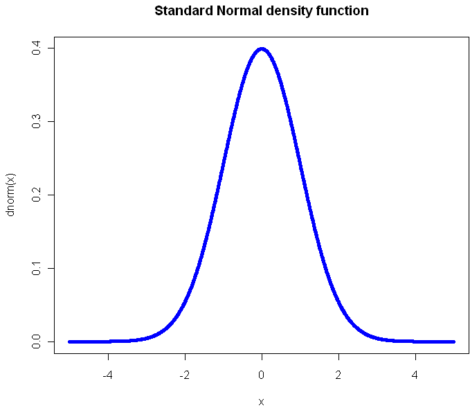
The standard, textbook way to represent a density function looks like this:

Perhaps you have seen this before? (Plot created in R, all source code from this post is included at the end). Not only will you find this plot in statistics books, you’ll also see it in medical texts, sociology, and even economics books. It gives you a clear view of how likely an observation is to fall in a particular range of [latex]x[/latex]. So what’s the problem?

The problem is that what usually concerns us isn’t probability in isolation. What matters is the impact that observations have on some other metric of importance, like the total or average. The key thing we want to know about a distribution is: What range of observations will contribute the most to our expected value, and in what way? We want a measure of influence.

Here’s the plot of the Cauchy density:

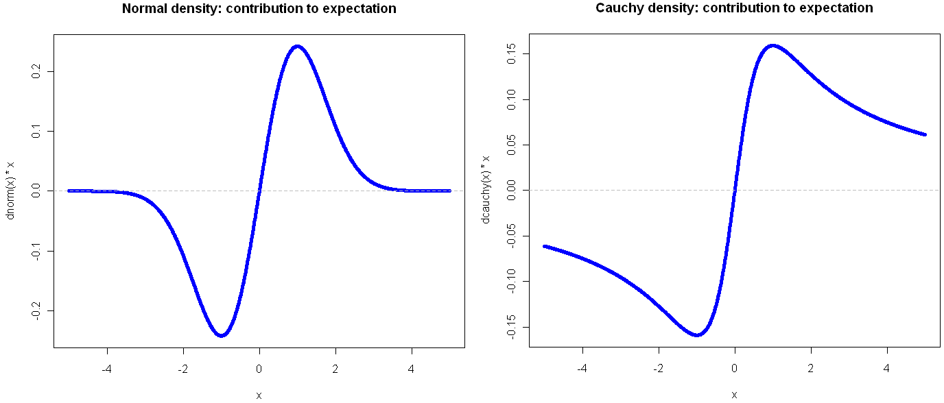
From this view, it doesn’t look all that different from the Normal. Sure it’s a little more narrow, with “fatter tails”, but no radical difference, right? Of course, the Cauchy is radically different from the normal distribution. Those slightly fatter tails give very little visual indication that the Cauchy is so extreme-valued that it has no expected value. Integrating to find the exception gives you infinity in both directions. If your distribution is like this, you’ve got problems and your plot should tell you that right away.

Here’s another way to visualize these two probability distributions:

Go ahead and click on the image above to see the full view. I’ll wait for you…

See? By plotting the density multiplied by the observation value on the y-axis, you get a very clear view of how the different ranges of the function effect the expectation. Looking at these, it should be obvious that the Cauchy is an entirely different beast. In the normal distribution, extreme values are so rare as to be irrelevant. This is why researchers like to find ways to treat their sample as normally distributed: a small sample gives enough information to tell the whole story. But if your life (or livelihood) depends on a sum or total amount, you’re probably best off plotting your (empirical) density in the way shown above.

Another bit of insight from this view is that the greatest contribution to the expectation comes at 1 and -1, which in the case of the Normal isn’t the mean, but rather the second central moment (plus or minus). That’s not a coincidence, but it’s also not always the case, as we shall see. But first, what do things look like when a distribution gets completely out of hand?

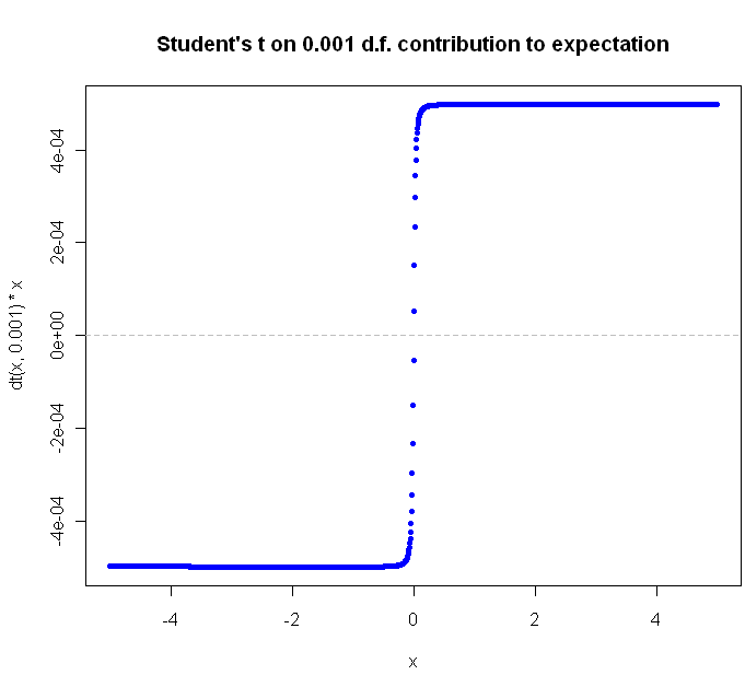
The Student’s t distribution, on 1 Degree of Freedom , is identical to the Cauchy. But why stop at a single DF? You can go all the way down to the smallest (positive) fraction.

The closer you get to zero, the flatter the curve gets. Can we ever flatten it out completely? Not for a continuous distribution with support over an infinite range. Why not? Because in order for the slope of [latex]value * density[/latex] to continue to flatline it indefinitely, the density function would have to be some multiple of [latex]\frac{1}{x}[/latex], and of course the area under this function diverges as we go to infinity, and densities are supposed to integrate to 1, not infinity, right?

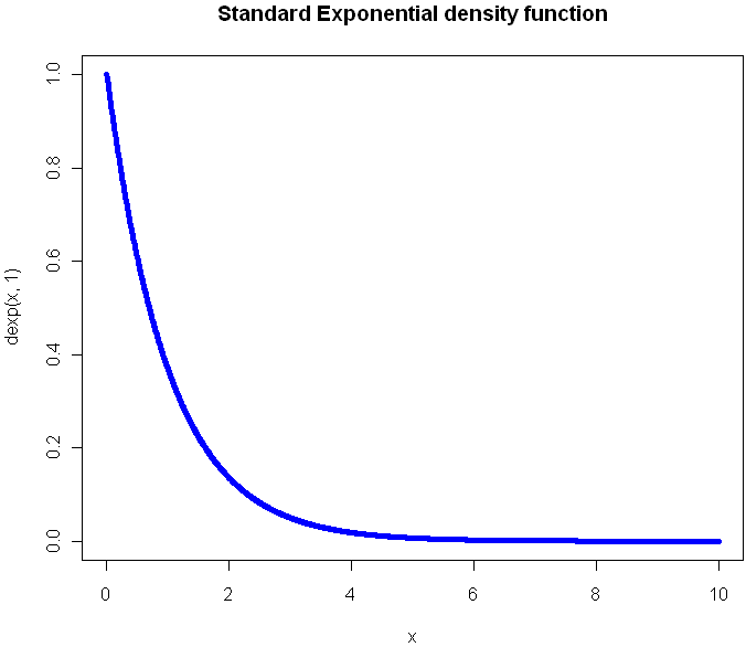
What would the plot look like for a continuous function that extends to infinity in just one direction? Here’s the regular Exponential(1) density function plot:

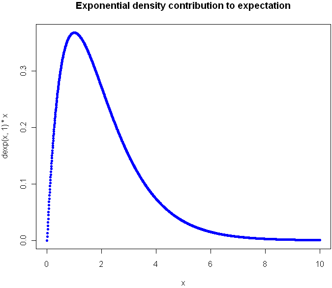
Now look at the plot showing contribution to expectation:

Were you guessing it would peak at 1?  Again, the expectation plot provides insight into which ranges of the distribution will have the greatest impact on our aggregate values.

Before I go look at an a discrete distribution, try to picture what the expectation curve would look like for the standard [latex]Uniform(0,1)[/latex] distribution. Did you picture a diagonal line?

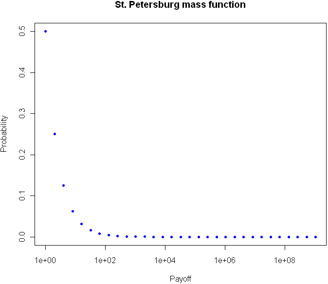
Can we flatten things out completely with an infinitely-supported discrete distribution? Perhaps you’ve heard of the St. Petersburg Paradox. It’s a gambling game that works like this: you flip a coin until tails comes up. If you see one head before a tails, you get $1. For 2 heads you get $2, for 3 heads $4, and so on. The payoff doubles each time, and the chances of reaching the next payoff are halved. The paradox is that even though the vast majority of your winnings will be quite modest, your expectation is infinite.  The regular view of the probability mass function for provides almost no insight:

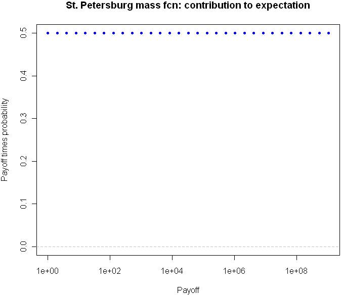
But take a look at the expectation plot:

Flat as a Nebraska wheat field. You can tell right away that something unusual is happening here.

I could go on with more examples, but hopefully you are beginning to see the value in this type of plot. Here is the code, feel free to experiment with other distributions as well.

# Useful way to make dots look like a line
x = seq(-5,5,length=1500)

# You've seen this before. Our good friend the Normal
plot(x,dnorm(x),pch=20,col="blue", main="Standard Normal density function")

# Cauchy looks a little different, but it's not obvious how different it is 
plot(x,dcauchy(x),pch=20,col="blue", main="Cauchy density function")

# New way of plotting the same
plot(x,dnorm(x)*x,pch=20,col="blue", main="Normal density: contribution to expectation")
abline(h=0,lty="dashed",col="gray")

plot(x,dcauchy(x)*x,pch=20,col="blue", main="Cauchy density: contribution to expectation")
abline(h=0,lty="dashed",col="gray")

# Extreme student-t action:
plot(x,dt(x,0.001)*x,pch=20,col="blue", main="Student's t on 0.001 d.f. contribution to expectation")
abline(h=0,lty="dashed",col="gray")


# The Exponential
x = seq(0,10,length=1500)
plot(x,dexp(x,1),pch=20,col="blue", main="Standard Exponential density function")

# The expectation view:
plot(x,dexp(x,1)*x,pch=20,col="blue", main="Exponential mass contribution to expectation")

# What do we see with the St. Petersburg Paradox
x = 2^(0:30)
dStPete <- function(x) {
	return (1/(2*x))
}

# Note the log
plot(x,dStPete(x),pch=20,col="blue", main="St. Petersburg mass function", log="x", xlab="Payoff", ylab="Probability",ylim=c(0,.5))

# Now we see the light
plot(x,dStPete(x)*x,pch=20,col="blue", main="St. Petersburg mass fcn: contribution to expectation", xlab="Payoff", log="x", ylab="Payoff times probability",ylim=c(0,.5))
abline(h=0,lty="dashed",col="gray")