feature
9
Jul 10
100 Prisoners, 100 lines of code
In math and economics, there is a long, proud history of placing imaginary prisoners into nasty, complicated scenarios. We have, of course, the classic Prisoner’s Dilemma, as well as 100 prisoners and a light bulb. Add to that list the focus of this post, 100 prisoners and 100 boxes.
In this game, the warden places 100 numbers in 100 boxes, at random with equal probability that any number will be in any box. Each convict is assigned a number. One by one they enter the room with the boxes, and try to find their corresponding number. They can open up to 50 different boxes. Once they either find their number or fail, they move on to a different room and all of the boxes are returned to exactly how they were before the prisoner entered the room.
The prisoners can communicate with each other before the game begins, but as soon as it starts they have no way to signal to each other. The warden is requiring that all 100 prisoners find their numbers, otherwise she will force them to listen to hundreds of hours of non-stop, loud rock musician interviews. Can they avoid this fate?
The first thing you might notice is that if every prisoner opens 50 boxes at random, they will have a [latex]0.5[/latex] probability of finding their number. The chances that all of them will find their number is [latex](\frac{1}2)^{100}[/latex], which is approximately as rare as finding a friendly alien with small eyes. Can they do better?
Of course they can. Otherwise I wouldn’t be asking the question, right? Before I explain how, and go into a Monte Carlo simulation in R, you might want to think about how they can do it. No Googling!
All set? Did you find a better way? The trick should be clear from the code below, but if not skip on to the explanation.
# How many times should we run this experiment?
iters = 1000
results = rep(0,iters)

for(i in 1:iters) {
	# A random permutation:
	boxes = sample(1:100,100)

	# Labels for our prisoners
	prisoners = 1:100

	# Track how many "winners" we have
	foundIt = 0

	# Main loop over the prisoners
	for(prisoner in prisoners) {

		# Track the prisoners path
		path = c(prisoner)

		tries = 1

		# Look first in the box that matches your own number
		inBox = boxes[prisoner]

		while(tries < 50) { 			 			path = c(path, inBox) 			 			if(inBox == prisoner) { 				#cat("Prisoner", prisoner, "found her number on try", tries, "\n") 				foundIt = foundIt + 1 				break; 			} else { 				# Follow that number to the next box 				inBox = boxes[inBox] 			} 			tries = tries+1 		} 		 		# cat("Prisoner", prisoner, "took path", paste(path, collapse=" -> "), "\n")
	}

	# How many prisoners found their numbers?
	cat("A total of", foundIt, "prisoners found their numbers.\n")
	flush.console()
	results[i] = foundIt
}

hist(results, breaks=100, col="blue")
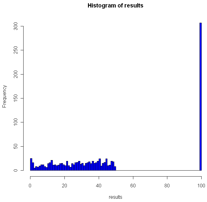
Here is what one of my plots looked like after running the code:
Out of the 1000 times I ran the experiment, on 307 occasions every single prisoner found his number. The theoretical success rate is about 31%. So, if it’s not clear from the code, what was the strategy employed by the prisoners and how does it work?
One way to look at the distribution of numbers in boxes is to see it as a permutation of the numbers from 1 to 100. Each permutation can be partitioned into what are called cycles. A cycle works like this: pick any number in your permutation. Let’s say it’s 23. Then you look at the number the 23rd place (ie the number in the 23rd box, counting from the left). If that number is 16, you look at the number in the 16th place. If that number is 87, go open box number 87 and follow that number. Eventually, the box you open up will have the number that brings you back to where you started, completing the cycle. Different permutations have different cycles.
The key for the prisoner is that by starting with the box that is the same place from the left as his number, and by following the numbers in the boxes, the prisoner guarantees that if he is in a cycle of length less than 50, he will eventually open the box with his number in it, which would complete the cycle he began. One way to envision cycles of different lengths is to think about the extreme cases. If a particular permutation shifted every single number over one to the left (and wrapped number 1 onto the end), you would have a single cycle of length 100. Box 1 would contain number 2, box 2 number 3 and so on. On the other hand, if a permutation flipped every pair of consecutive numbers, you would have 50 cycles, each of length 2: box 1 would have number 2, box 2 would have number 1. Of course if your permutation doesn’t change anything you have 100 cycles of length 1.
As you can see from the histogram, when using this strategy you can never have between 50 and 100 winning prisoners. Anytime you have a single cycle of length greater than 50, for example 55, then all 55 prisoners who start on that cycle will fail to find their number. If no cycles are longer than 50, everyone wins. Just how rare are different cycles of different lengths? For the math behind that check out this excellent explanation by Peter Taylor of Queen’s University.
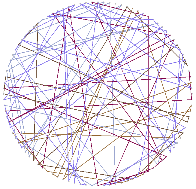
Before moving on I wanted to visualize these cycles. Try running the code below:
# Unit circle
plot(0,0,xlim=c(-1,1),ylim=c(-1,1),col="white",ann=FALSE, xaxt="n", yaxt="n")
for(i in 1:100) {
	points(cos(2*i/100*pi), sin(2*i/100*pi),pch=20,col="gray")
}

mySample = sample(1:100,100)
for(i in 1:100) {
	found = FALSE
	nextItem = i

	# Pick a random color for this cycle
	color = sample(c(0:9,"A","B","C","D","E","F"),12,replace=T)
	lineColor = paste("#", paste(color[1:6],collapse=""),sep="")

	while(!found) {
		# Draw the cycle

		segments(cos(nextItem/50*pi), sin(nextItem/50*pi), cos(mySample[nextItem]/50*pi), sin(mySample[nextItem]/50*pi),col=lineColor,lwd=2)
		Sys.sleep(.4)
		if(mySample[nextItem] == i) {
			found = TRUE
		} else {
			nextItem = mySample[nextItem]
		}
	}
}
You can adjust the “Sys.sleep()” parameter to make the animation faster. I recommend running the code to see how the cycles “develop” over time, but here’s a snapshot of what I got:
2
Jul 10
Word games in probability and R
Last night, while playing Boggle, we ended up with a board without a single vowel. Not even a “Y” or “Qu”. This seemed fairly unusual, so I wondered what the chances were of such an occurrence. I found an online list of the letters each die has, and I could have written down the number of vowels on each one by hand, but whenever possible I like to do things by computer. So I fired up Hal and asked for some help with the calculations.
Apparently some European boards use a 5 x 5 grid, but here in the land of the Maple leaf our board has 16 cubes. Here are the letters on them, as I coded them into R:
d1 = c('S','R','E','L','A','C')
d2 = c('D','P','A','C','E','M')
d3 = c('Qu','B','A','O','J','M')
d4 = c('D','U','T','O','K','N')
d5 = c('O','M','H ','R','S','A')
d6 = c('E','I','F','E','H','Y')
d7 = c('B','R','I','F','O','X')
d8 = c('R','L','U','W','I','G')
d9 = c('N','S','O','W','E','D')
d10 = c('Y ','L','I','B','A','T')
d11 = c('T','N','I','G','E','V')
d12 = c('T','A','C','I','T','O')
d13 = c('P','S','U','T','E','L')
d14 = c('E','P','I','S','H ','N')
d15 = c('Y','K','U','L','E','G')
d16 = c('N','Z','E','V','A','D')
So now I had to check how many vowels were on each die. Here’s the code I used for this:
vowels = c('A','E','I','O','U','Qu','y')
vowelsFound = rep(0,16)
for(i in 1:16) {
	found = 0
	die = eval(parse(text=paste("d",i,collapse="",sep="")))
	for(l in die) {
		# Check to see if this letter is in the vowels vector
		if(l %in% vowels) {
			found = found + 1
		}
	}
	vowelsFound[i] = found
}

# Probabilities of getting a vowel for each die
pVowels = vowelsFound/6

# Probability of getting no vowel for each die
pNoVowels = 1 - pVowels

# Chance that we will get not a single vowel, including "y" and "Qu"
print(prod(pNoVowels))
If you run the code above, you should see that the probability of getting no vowels (including “Y” and “Qu”) is 0.000642. That works out to one in every 1557 boards. So it’s quite rare, but by no means so extraordinary that it crosses the Universal probability bound. Also, it’s not enough to just calculate how rare your event is, or how rare any similar or more extreme event is, and then be astounded. You also have to include all the other possible events that would have left you amazed. What about getting all vowels (much more rare)? What about getting 8 or 9 E’s, or a row or column of all A’s or E’s? It’s likely that if you add up all probabilities of all the rare events which might leave you amazed, you’ll end up with a good chance of amazement every time.
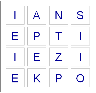
I could have stopped here, but having coded the dice, I decided to create a simplified version of the game in R. If I have a chance over the next few days I’ll add some more features.
# You will need to download a dictionary file. I found one here:
# http://svn.pietdepsi.com/repos/projects/zyzzyva/trunk/data/words/north-american/owl2-lwl.txt
words = read.table("wordlistData.dat", colClasses = "character")
words = unlist(words[,1])

# Create a random board. Plot it.
board = diag(4)
dice = sample(1:16,16)
cntr = 4
for(i in dice) {
	die = eval(parse(text=paste("d",i,collapse="",sep="")))
	board[floor(cntr/4), (cntr %% 4) + 1] = sample(die,1)
	cntr = cntr + 1
}

plot(0,0,xlim=c(0,4),ylim=c(0,4),col="white",ann=FALSE, xaxt="n", yaxt="n" )

for(m in 1:4) {
	for(n in 1:4) {
		text(m-.5,n-.5,labels=board[m,n],cex=2.75,col="#000099")
		# Draw a square the easy way
		points(m-.5,n-.5,pch=0,cex=10,lwd=1.5,col="gray")
	}
}

# How many seconds to give for each round
gameTime = 180

START_TIME = proc.time()[3]
elapsed = 0

# Simple scoring, with 1 point per letter.
# Dictionary only has words length 3 or longer
score = 0

cat("Find words. Hit enter after each word.\n")
while(elapsed < gameTime) {
	myWord = scan(n=1, what=character()) # Get a single word
	elapsed = signif(proc.time()[3] - START_TIME, digits=4)
	if (length(myWord)==0) {
		cat("You have", gameTime - elapsed, "seconds left. Keep going!\n")
	} else {

		if(elapsed < gameTime) {
			# Check if it's a real word, see if it is in dictionary
			# Convert their guess to uppercase letter
			myWord = toupper(myWord)

			# If it is in the dictionary, give them points
			if(myWord %in% words) {
				# Make sure they haven't used this word before TODO

				# Add it to their score
				score = score + nchar(myWord)
				cat("Congratulations. You are up to", score, "points.")
				cat("You have", gameTime - elapsed, "seconds left. Keep going!\n")
			} else {
				# If it isn't in the dictionary, let the user know that they got it wrong.
				cat("Sorry, that is not in the dictionary. Keep trying!\n")
			}


		}
	}
}

cat("Out of time! ")
cat("Your final score was:", score, "points.")
Enjoy the game. Let me know if you notice any issues or have suggestions!
29
Jun 10
Entropy augmentation the modulo way
Long before I had heard about the connection between entropy and probability theory, I knew about it from the physical sciences. This is most likely how you met it, too. You heard that entropy in the universe is always increasing, and, if you’re like me, that made very little sense. Then you may have heard that entropy is a measure of disorder: over times things fell apart. This makes a little more sense, especially to those teenagers tasked with cleaning their own rooms. Later on, perhaps you got a more precise, mathematical definition of entropy that still didn’t fully mesh with the world as we observe it. Here on earth, we see structures getting built up over time: plants convert raw energy to sunflowers, bees build honeycombs, humans build roads. Things do sometimes fall apart. More precisely, levels of complexity tend to grow incrementally over long periods of time, then collapse very quickly. This particular asymmetry seems to be an ironclad rule for our word, which I assume everyone understands, at least implicitly, though I can’t remember anywhere this rule is written down as such.
In the world of probability, entropy is a measure of unpredictability. Claude Shannon, who created the field of Information Theory, gave us an equation to measure how much, or little, is known about an incoming message a prori. If we know for sure exactly what the message will be, our entropy is 0. There is no uncertainty. If we don’t know anything about the outcome except that it will be one of a finite number of possibilities, we should assume uniform probability for any one of the outcomes. Uncertainty, and entropy, is maximized. The more you look into the intersection of entropy and statistics, the more you find surprising, yet somehow obvious in retrospect, connections. For example, among continuous distributions with fixed mean and standard deviation, the Normal distribution has maximal entropy. Surprised? Think about how quickly a sum of uniformly distributed random variables converges to the Normal distribution. Better yet, check it out for yourself:
n = 4
tally = rep(0,10000)
for(i in 1:n) {
	tally = tally + runif(10000)
}

hist(tally, breaks=50, col="blue")
Try increasing and decreasing “n” and see how quickly the bell curve begins to appear.
Lately I’ve been thinking about how to take any general distribution and increase the entropy. The method I like best involves chopping off the tails and “wrapping” these extreme values back around to the middle. Here’s the function I created:
smartMod <- function(x, mod) {
	sgn = sign(x)
	x = abs(x)
	x = x %% mod
	return(sgn * x)
}
Now is a perfect time to use a version of our “perfect sample” function:
perfect.sample <- function(dist, n, ...) {
	match.fun(paste('q', dist, sep=''))((1:n) / (n+1), ...)
}
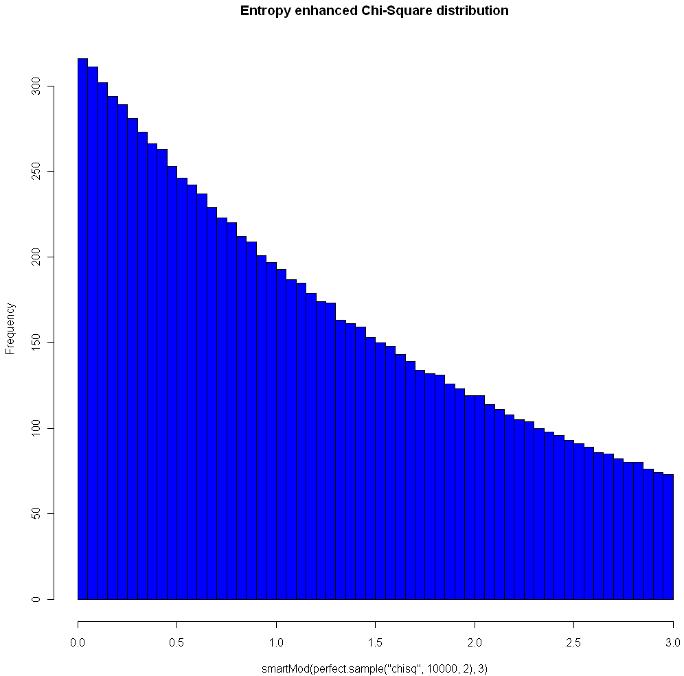
The image at the top of this post shows the Chi Square distribution on 2 degrees of freedom, with Modulo 3 Entropy Enhancement (see how nice that sounds?). Here’s the code to replicate the image:
hist(smartMod(perfect.sample("chisq",10000,2),3),breaks=70,col="blue",main="Entropy enhanced Chi-Square distribution")
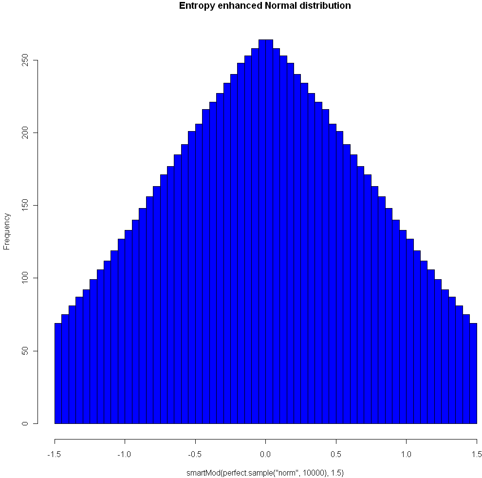
Here’s another plot, using the Normal distribution and Modulo 1.5:
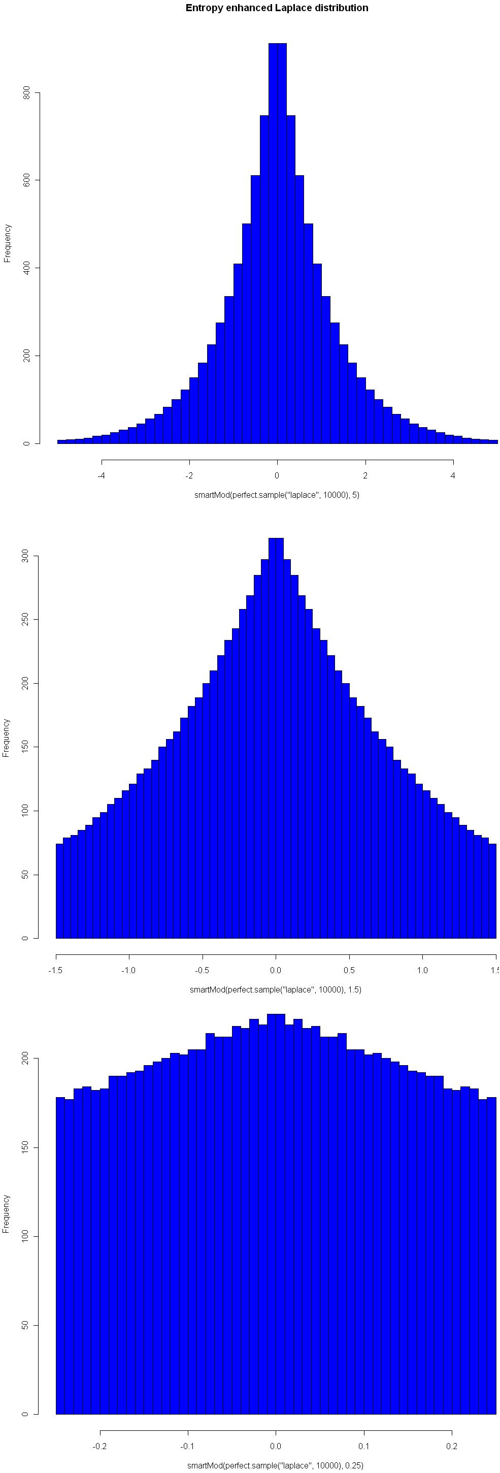
One nice property of this method of increasing entropy is that you get a smooth transition with logical extremes: As your choice of Mod goes to infinity, the distribution remains unchanged. As your Mod number converges to 0, entropy (for that given width) is maximized. Here are three views of the Laplace, with Mods 5, 1.5, and 0.25, respectively. See how nicely it flattens out? (Note you will need the library “VGAM” to sample from the Laplace).
It’s not clear to me yet how entropy enhancement could be of practical use. But everyone loves enhancements, right? And who among us doesn’t long for a little extra entropy for time to time, no?
26
Jun 10
Weekend art in R (Part 2)
I put together four of the best looking images generated by the code shown here:
# More aRt
par(bg="white")
par(mar=c(0,0,0,0))
plot(c(0,1),c(0,1),col="white",pch=".",xlim=c(0,1),ylim=c(0,1))
iters = 500
for(i in 1:iters) {
	center = runif(2)
	size = 1/rbeta(2,1,3)

	# Let's create random HTML-style colors
	color = sample(c(0:9,"A","B","C","D","E","F"),12,replace=T)
	fill = paste("#", paste(color[1:6],collapse=""),sep="")
	brdr = paste("#", paste(color[7:12],collapse=""),sep="")

	points(center[1], center[2], col=fill, pch=20, cex=size)
	points(center[1], center[2], col=fill, pch=21, cex=size,lwd=runif(1,1,4))
}
Weekend art Part 1 is here.
25
Jun 10
A rare event in tennis
70-68
That was the final score in the final set, won by John Isner over Nicolas Mahut at Wimbledon. In the final set of a match the winner has to beat the other by at least 2 games, so as in baseball matches can (theoretically) go on indefinitely. In practice even final sets that go into “extra innings” tend to end quickly. The previous record for number of games in a final set was 1/3 as many. For some commentary on the odds related to this extraordinary match check out:
A mathematician watches tennis II
Wikipedia has a list of Longest tennis match records.
23
Jun 10
Data is dumb, try to be smart
I blurred out my personal information, but otherwise the check shown above is exactly as I received it. Yahoo! really did send me a check for ZERO DOLLARS 00 CENTS. Obviously, mailing out checks for nothing is wasteful and pointless (shall I try cashing it? Will the bank “credit” me for nothing?). It could be that this check isn’t even “legal”, if I’m to believe the Best Answer by Yahoo!’s crack team of expert volunteers. But instead of making this a “Ha! Ha! Big Company Does Something Stupid” post, I thought I’d dig a little deeper into the story behind the check.
Until recently, Yahoo! had an advertising program similar to Google’s Adsense. Webmasters could show ads from Yahoo!’s network and share in the profits when people clicked on the links. Although basically similar, Yahoo!’s version was much more restrictive: fewer websites were accepted into their network and webmasters could only display ads to visitors from the United States. I can understand why Yahoo! would want to limit payment to clicks coming from a single (huge and wealthy) country, but the way they implemented this requirement struck me as odd. It was the webmaster’s responsibility to make sure no one from outside the US saw their ads. This meant that I had to install Geo-IP software on my server, which maps the unique numerical identifiers of visitors to their country of origin. Installing this software is a pain, and you have to update it regularly with the latest free or paid versions of the database, or else the information becomes inaccurate. Yahoo!, with all its infrastructure and CPU power and economies of scale, was making thousands of individual webmasters perform a task best handled by a giant IT company, like, say, Yahoo!
The other strange, and occasionally frustrating, thing about Yahoo!’s program was the high volatility in payment amounts. On average, the earnings from their ad network were good, but I would see days when a website made $50 and others when it made $2.11, sometimes from the same number of visitors or even the same number of clicks. Variability is built in to programs like this, but I found Yahoo!’s results to be way more inconsistent that Google’s or even some of the much smaller companies with their own advertising networks. You might think that only the average matters, but high volatility leads to poorer decision making. Imagine the following two scenarios: in one, you see the revenue from a advertising program slowly and steadily decline over the course of months. Time to find a different program. In the other scenario, payouts vary widely from month to month. Some are fantastic, some very poor. How can you tell when to leave the program, and when to expand your use of it? There are ways to measure non-obvious trends with time series analysis. But no matter which tool you use, the more “noise” in your data stream, the worse your predictions will be.
High volatility in Yahoo!’s payouts was so prolonged that it couldn’t have been just a matter of growing pains. Either no-one at Yahoo! was looking into payment variability at the level of individual users (it’s possible that the total revenue generated by their program, summed across all users, was much more stable), or they didn’t see why this was a problem.
Finally, we have the issue of the worthless check. When Yahoo! closed their program, they had to send out final checks, even to those users with balances below the regular minimum threshold (most programs require $50 or so in earnings before they send you a check). One possibility is that Yahoo!’s algorithm never looked to see if the amount owed was positive before cutting a check. That would be really dumb. Another, slightly-more-favorable explanation is that they really owed me 0.5 cents, so their algorithm saw this as a positive balance. It looked like I should be getting a check, but then Yahoo!’s check-printing software rounded down to the nearest penny and I end up with $0.00. Either way, I see this as a final indicator that Yahoo! just isn’t thinking very hard about their data. By contrast, Google and other companies seem to understand that their business depends on managing data with a huge amount of human intelligence and understanding. Data is dumb, Yahoo! needs to be smarter.
22
Jun 10
Reaching escape velocity
Sample once from the Uniform(0,1) distribution. Call the resulting value [latex]x[/latex]. Multiply this result by some constant [latex]c[/latex]. Repeat the process, this time sampling from Uniform(0, [latex]x*c[/latex]). What happens when the multiplier is 2? How big does the multiplier have to be to force divergence. Try it and see:
iters = 200
locations = rep(0,iters)
top = 1
multiplier = 2
for(i in 1:iters) {
	locations[i] = runif(1,0,top)

	top = locations[i] * multiplier
}

windows()
plot(locations[1:i],1:i,pch=20,col="blue",xlim=c(0,max(locations)),ylim=c(0,iters),xlab="Location",ylab="Iteration")

# Optional save as movie, not a good idea for more than a few hundred iterations. I warned you!
# library("animation")
# saveMovie(for (i in 1:iters) plot(locations[1:i],1:i,pch=20,col="blue",xlim=c(0,max(locations)),ylim=c(0,iters),xlab="Location",ylab="Iteration"),loop=1,interval=.1)
19
Jun 10
The perfect fake
Usually when you are doing Monte Carlo testing, you want fake data that’s good, but not too good. You may want a sample taken from the Uniform distribution, but you don’t want your values to be uniformly distributed. In other words, if you were to order your sample values from lowest to highest, you don’t want them to all be equidistant. That might lead to problems if your underlying data or model has periods or cycles, and in any case it may fail to provide correct information about what would happen with real data samples.
However, there are times when you want the sample to be “perfect”. For example, in systematic sampling you may wish to select every 10th object from a population that is already ordered from smallest to biggest. This method of sampling can reduce the variance of your estimate without introducing bias. Generating the numbers for this perfect sample is quite easy in the case of the Uniform distribution. For example, R gives you a couple easy ways to do it:
# Generate a set of 100 equidistant values between 5 and 10 (inclusive)
x <- seq(5,10,length=100)

# Generate every 12th integer between 50 and 1000
x <- seq(50,1000,12)
When it comes to other distributions, grabbing a perfect sample is much harder. Even people who do a lot of MC testing and modeling may not need perfect samples every day, but it comes up often enough that R should really have the ability to do it baked right into to the language. However, I wasn't able to find such a function in R or in any of the packages, based on my searches at Google and RSeek. So what else could I do but roll my own?
# Function returns a "perfect" sample of size n from distribution myDist
# The sample is based on uniformly distributed quantiles between 0 and 1 (exclusive)
# If the distribution takes additional parameters, these can be specified in the vector params
# Created by Matt Asher of StatisticsBlog.com
perfect.sample <- function(n, myDist, params = c()) {
	x <- seq(0,1,length=(n+2))[2:(n+1)]

	if(length(params)) {
	  	toEval <- paste(c("sapply(x,q", myDist, ",", paste(params,collapse=","), ")"), collapse="")
	} else {
	  	toEval <- paste(c("sapply(x,q", myDist, paste(params,collapse=","), ")"), collapse="")
	}

	eval(parse(text=toEval))
}
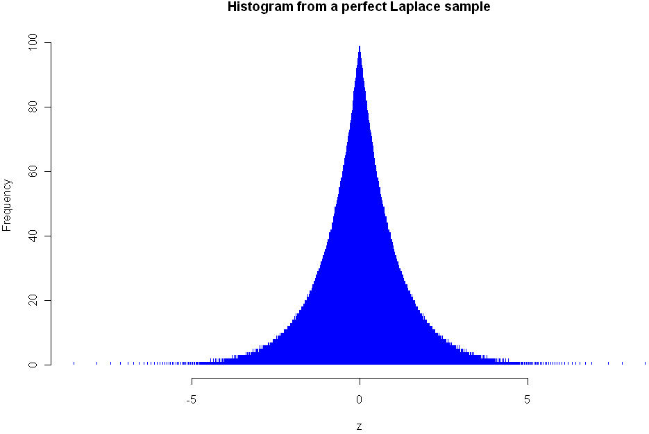
This function should work with any distribution that follows the naming convention of using "dname" for the density of the distribution and has as its first parameter the number of values to sample. The histogram at the top of this post shows the density of the Lapalce, aka Double Exponential distribution. Here is the code I used to create it:
# Needed library for laplace
library(VGAM)
z <- perfect.sample(5000,"laplace",c(0,1))
hist(z,breaks=800,col="blue",border=0,main="Histogram from a perfect Laplace sample")
As you can see, my function plays nice with distributions specified in other packages. Here are a couple more examples using standard R distributions:
# Examples:
perfect.sample(100,"norm")

# Sampling from the uniform distribution with min=10 and max=20
z <- perfect.sample(50,"unif",c(10,20))
Besides plotting the results with a histogram, there are specific tests you can run to see if values are consistent with sampling from a known distribution. Here are tests for uniformity and normality. You should get a p-value of 1 for both of these:
# Test to verify that this is a perfect sample, requires library ddst
# Note only tests to see if it is Uniform(0,1) distributed
library(ddst)
ddst.uniform.test(z, compute.p=TRUE)

# Needed for the Shapiro-Wilk Normality Test
library(stats)
z = perfect.sample(1000,"norm")
shapiro.test(z)
If you notice any bugs with the "perfect.sample" function please let me know. Also let me know if you find yourself using the function on a regular basis.
18
Jun 10
Those dice aren’t loaded, they’re just strange
I must confess to feeling an almost obsessive fascination with intransitive games, dice, and other artifacts. The most famous intransitive game is rock, scissors, paper. Rock beats scissors. Scissors beats paper. Paper beats rock. Everyone older than 7 seems to know this, but very few people are aware that dice can exhibit this same behavior, at least in terms of expectation. Die A can beat die B more than half the time, die B can beat die C more than half the time, and die C can beat die A more than half the time.
How is this possible? Consider the following three dice, each with three sides (For the sake of most of this post and in my source code I pretend to have a 3-sided die. If you prefer the regular 6-sided ones, just double up every number. It makes no difference to the probabilities or outcomes.):
Die A: 1, 5, 9
Die B: 3, 4, 8
Die C: 2, 6, 7
Die A beats B [latex]5/9[/latex] of the time which beats C [latex]5/9[/latex] of the time which beats A [latex]5/9[/latex] of the time. Note that the ratios don’t all have to be the same. Here’s another intransitive trio:
Die A: 2, 4 ,9
Die B: 1, 8, 7
Die C: 3, 5, 6
Take a moment to calculate the relative winning percentages, or just trust me that they are not all the same…. Did you trust me? Will you trust me now in the future?
In order to find these particular dice I wrote some code in R to automate the search. The following functions calculate the winning percentage for one die over another and check for intransitivity:
# Return the proportion of the time that d1 beats d2.
# Dice need to have same number of sides
calcWinP <- function(d1,d2) {
	sides = length(d1)
	d1Vd2 = 0

	for(i in 1:sides) {
		for(j in 1:sides) {
			if(d1[i] > d2[j]) {
				d1Vd2 = d1Vd2 + 1
			}
		}
	}

	return( d1Vd2/(sides^2) )
}

# Assumes dice have no ties.
# All dice must have the same number of sides.
# How many times do I have to tell you that?
checkIntransitivity <- function(d1,d2,d3) {
	d1beatsd2 = calcWinP(d1,d2)

	if (d1beatsd2 > 0.5) {
		if(calcWinP(d2,d3) > 0.5) {
			if(calcWinP(d3,d1) > 0.5) {
				return(TRUE)
			}
		}
	} else {
		# Check if d1 beats d3, if so check if d3 beats d2
		if(calcWinP(d1,d3) > 0.5) {
			if(calcWinP(d3,d2) > 0.5) {
				return(TRUE)
			}
		}
	}
	# Regular old transitivity.
	return(FALSE)
}
I then checked every possible combination. How many unique configurations are there? Every die has three numbers on it, and you have three die for a total of nine numbers. To make things simpler and avoid ties, no number can be used more than once. If each sides of a die was ordered and each of the die was ordered, you’d have [latex]9![/latex] different combinations, which is to say a whole mess of them. But our basic unit of interest here isn’t the digits, it’s the dice. So let’s think about it like this: For die A you can choose 6 of the 9 numbers, for die B you can pick 3 of the remaining 6, and for die C you’re stuck with whatever 3 are left. Multiply this all together:
choose(9,6)*choose(6,3)
and you get 1680 possibilities. But wait? What’s that you say? You don’t care which die is A, which is B, and which is C? Fantastic. That reduces the number of “unique” configurations by [latex]3![/latex], which is to say 6, at least if my back-of-the-envelope calculations are correct. Final tally? 280.
Not bad. Unfortunately, there no obvious way to ennumerate each of these 280 combinations (at least not to me there isn’t). So I ended up using a lot of scratch work and messing around in the R console until I had what I believed to be the right batch. Sorry, I no longer have the code to show you for that. After testing those 280 configurations, I found a total of 5 intransitive ones, including the 2 dice shown previously and the following 3 sets:
Die A: 2, 9, 3
Die B: 1, 6, 8
Die C: 4, 7, 5
Die A: 7, 1, 8
Die B: 5, 6, 4
Die C: 9, 3, 2
Die A: 7, 3, 5
Die B: 2, 9, 4
Die C: 8, 6, 1
Did I make a mistake? According to my calculations, [latex]5/280[/latex] of the combinations are intransitive. That represents 1.786% of the total. How might I very this? That’s right, it’s Monte Carlo time.
Using the following code, I created all [latex]9![/latex] permutations of dice and sides, then sampled from those 362,880 sets of dice many, many times:
library(e1071) # Makes making permutations easy
allPerms = permutations(9)
intransFound = 0
for(i in 1:dim(allPerms)[1]) {
	d1 = allPerms[i,1:3]
	d2 = allPerms[i,4:6]
	d3 = allPerms[i,7:9]
	if(checkIntransitivity(d1,d2,d3)) {
		intransFound = intransFound + 1
	}
}

print(intransFound)

found = 0
tries = 100000
for(i in 1:tries) {
	one2nine = sample(1:9,9)
	d1 = one2nine[1:3]
	d2 = one2nine[4:6]
	d3 = one2nine[7:9]

	if( checkIntransitivity(d1,d2,d3)) {
		found = found + 1
		# Uncomment below if you want to see them.
		#print("found one")
		#print(d1)
		#print(d2)
		#print(d3)
		#flush.console()
	}
}

print(found/tries)
Final percentage: 1.807%. That’s pretty close to [latex]5/280[/latex], and much closer than it is to either [latex]4/280[/latex] or [latex]6/280[/latex], so I’m going to conclude that I got them all and got it right.
What happens if your dice have fewer, or more, sides? Turns out you need at least 3 sides to achieve intransitivity. Can you have it with 4 sides? What about 5, 6, or 7? To estimate the fraction of dice configurations which are intransitive for different numbers of sides I wrote the following code. Note that this could take a while to run, depending on the number of “tires” you use:
# Transitivity vs sides.
results = rep(0,6)
tries = 100000

for(j in 4:12) {
	found = 0

	for(i in 1:tries) {
		one2nine = sample(1:(3*j),(3*j))
		d1 = one2nine[1:j]
		d2 = one2nine[(j+1):(2*j)]
		d3 = one2nine[(2*j+1):(3*j)]

		if( checkIntransitivity(d1,d2,d3)) {
			found = found + 1
		}
	}

	results[j] = found/tries
	print("Found:")
	print(results[j])
	flush.console()
}
If you wait through all that you might notice some interesting patters emerge, which probably have explanations rooted in theory but it’s getting on nap time, so I’ll wrap this post up.
I think what fascinates me the most about intransitive dice, and games like rock, scissors, paper, is that they represent breakdowns in what math folks like to call a “total order”. Most of our calculations are done in this nice land of numbers where you can count on transitivity. [latex]A>B[/latex] and [latex]B>C[/latex], therefore [latex]A>C[/latex]. Every item has it’s place on the hierarchy, and “ties” only occur between an object and itself. “Total order” is a good name in that these are comfortable spaces to do calculations where nothing all that unexpected happens (usually, ok?). For excitement and unexpected delight, you need relax those orders, the more relaxing the better. Incidentally, if instead your goal is frustration and dirty looks from your friends at a party, try pretending that you can apply the methods of a total order (like the calculus) to economics, consumer choice, and love.
One final note before drifting off… in statistics we have at least one delightfully unexpected instance of intransitivity: correlations. Just because [latex]X[/latex] is positively correlated with [latex]Y[/latex] and [latex]Y[/latex] is positively correlated with [latex]Z[/latex], doesn’t mean that [latex]X[/latex] and [latex]Z[/latex] are positively correlated. Strange, no? But you can prove it with an example covariance matrix. Have you got one to show me?


