Posts Tagged: simulations


11
Dec 14

Can pregnant women intuit the sex of their children?

“So let’s start with the fact that the study had only 100 people, which isn’t nearly enough to be able to make any determinations like this. That’s very small power. Secondly, it was already split into two groups, and the two groups by the way have absolutely zero scientific basis. There is no theory that says that if I want a girl or if I want a boy I’m going to be better able at determining whether my baby is in fact a girl or a boy.”

– Maria Konnikova, speaking on Mike Pesca’s podcast, The Gist.

Shown at top, above the quote by Konnikova, is a simulation of the study in question, under the assumption that the results were completely random (the null hypothesis). As usual, you’ll find my code in R at the bottom. The actual group of interest had just 48 women. Of those, 34 correctly guessed the sex of their gestating babies. The probability that you’d get such an extreme result by chance alone is represented by the light green tails. To be conservative, I’m making this a two-tailed test, and considering the areas of interest to be either that the women were very right, or very wrong.

The “power” Konnikova is referring to is the “power of the test.” Detecting small effects requires a large sample, detecting larger effects can be done with a much smaller sample. In general, the larger your sample size, the more power you have. If you want to understand the relationship between power and effect size, I’d recommend this lovely video on the power of the test.

As it turns out, Konnikova’s claims notwithstanding, study authors Victor Shamas and Amanda Dawson had plenty of power to detect what turns out to be a very large effect. Adding together the two green areas in the tails, their study has a p-value of about 0.005. This a full order of magnitude beyond the generally used threshold for statistical significance. Their study found strong evidence that women can guess the sex of their babies-to-be.

Is this finding really as strong as it seems? Perhaps the authors made some mistake in how they setup the experiment, or in how they analyzed the results.

Since apparently Konnikova failed not only to do statistical analysis, but also basic journalism, I decided to clean up on that front as well. I emailed Dr. Victor Shamas to ask how the study was performed. Taking his description at face value, it appears that the particular split of women into categories was based into the study design; this wasn’t a case of “p-value hacking”, as Konnikova claimed later on in the podcast.

Konnikova misses the entire point of this spit, which she says has “absolutely zero scientific basis.” The lack of an existing scientific framework to assimilate the results of the study is meaningless, since the point of the study was to provide evidence (or not) that that our scientific understanding lags behind what woman seem to intuitively know.

More broadly, the existence of causal relationships does not depend in any way on our ability to understand or describe (model) them, or on whether we happen to have an existing scientific framework to fit them in. I used to see this kind of insistence on having a known mechanism as a dumb argument made by smart people,  but I’m coming to see it in a much darker light. The more I learn about the history of science, the more clear it becomes that the primary impediment to the advancement of science isn’t the existence of rubes, it’s the supposedly smart, putatively scientific people who are unwilling to consider evidence that contradicts their worldview, their authority, or their self-image. We see this pattern over and over, perhaps most tragically in the unwillingness of doctors to wash their hands until germ theory was developed, despite evidence that hand washing led to a massive reduction in patient mortality when assisting with births or performing operations.

Despite the strength of Shamas and Dawson’s findings, I wouldn’t view their study as conclusive evidence of the ability to “intuit” the sex of your baby. Perhaps their findings were a fluke, perhaps some hidden factor corrupted the results (did the women get secret ultrasounds on the sly?). Like any reasonable scientist, Shamas wants to do another study to replicate the findings, and told me that has a specific follow-up in mind.

Code in R:

trials = 100000
results = rep(0,trials)
for(i in 1:trials) {
	results[i] = sum(sample(c(0,1),48,replace=T))
}

extremes = length(results[results<=14]) + length(results[results>=34]) 
extremes/trials

dat <- data.frame( x=results, above=((results <= 14) | (results >= 34)))
library(ggplot2)
qplot(x,data=dat,geom="histogram",fill=above,breaks=seq(1,48))

20
Oct 11

Queueing up in R, continued

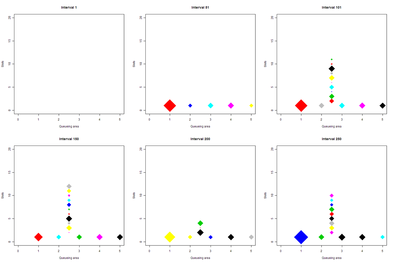
Shown above is a queueing simulation. Each diamond represents a person. The vertical line up is the queue; at the bottom are 5 slots where the people are attended to. The size of each diamond is proportional to the log of the time it will take them to be attended. Color is used to tell one person from another and doesn’t have any other meaning. Code for this simulation, written in R, is here. This is my second post about queueing simulation, you can find the first one, including an earlier version of the code, here. Thanks as always to commenters for their suggestions.

A few notes about the simulation:

  • Creating an animation to go along with your simulation can take a while to program (unless, perhaps, you are coding in Flash), and it may seem like an extra, unnecessary step. But you can often learn a lot just by “watching”, and animations can help you spot bugs in the code. I noticed that sometimes smaller diamonds hung around for much longer then I expected, which led me to track down a tricky little error in the code.
  • As usual, I’ve put all of the configuration options at the beginning of the code. Try experimenting with different numbers of intervals and tellers/slots, or change the mean service time.
  • If you want to run the code, you’ll need to have ImageMagick installed. If you are on a PC, make sure to include the full path to “convert”, since Windows has a built-in convert tool might take precedence. Also, note how the files that represent the individual animation cells are named. That’s so that they are added in the animation in the right order, naming them sequentially without zeros at the beginning failed.
  • I used Photoshop to interlace the animated GIF and resave. This reduced the file size by over 90%
  • The code is still a work in progress, it needs cleanup and I still have some questions I want to “ask” of the simulation.

12
Jan 11

R: Attack of the hair-trigger bees?

In their book “Complex Adaptive Systems”, authors Miller and Page create a theoretic model for bee attacks, based on the real, flying, honey-making, photogenic stingers. Suppose the hive is threatened by some external creature. Some initial group of guard bees sense the danger and fly off to attack. As they go, they lay down a scent. Other bees join in the attack if their scent sensitivity threshold (SST) is reached. When they join the attack, they send out their own warning scent, perhaps triggering an even bigger attack. The authors make the point that if the colony of bees were homogeneous, and every single one had the same attack threshold, then if that threshold was above the initial attack number, then no one else would join in. If it were below, then everyone goes all at once. Fortunately for the bees, they are a motley lot, which is to say a lot more diverse than you would imagine just from looking at the things. As a result, they exhibit much more complicated behavior. The authors describe a model with 100 bees and call their attack threshold “R”. By assuming a heterogeneous population of 100 with thresholds all equal spaced, they note:

“In the hetrogeneous case, a full-scall attack ensues for [latex]R \geq 1[/latex]. This latter result is easy to see, because once at least one bee attacks, then the bee with threshold equal to one will join the fray, and this will trigger the bee with the next highest threshold to join in, and so on…. It is relatively difficult to get the homogeneous hive to react, while the hetrogeneous one is on a hair trigger. Without explicity incorporating the diversity of thresholds, it is difficult to make any kind of accurate prediction of how a given hive will behave.”

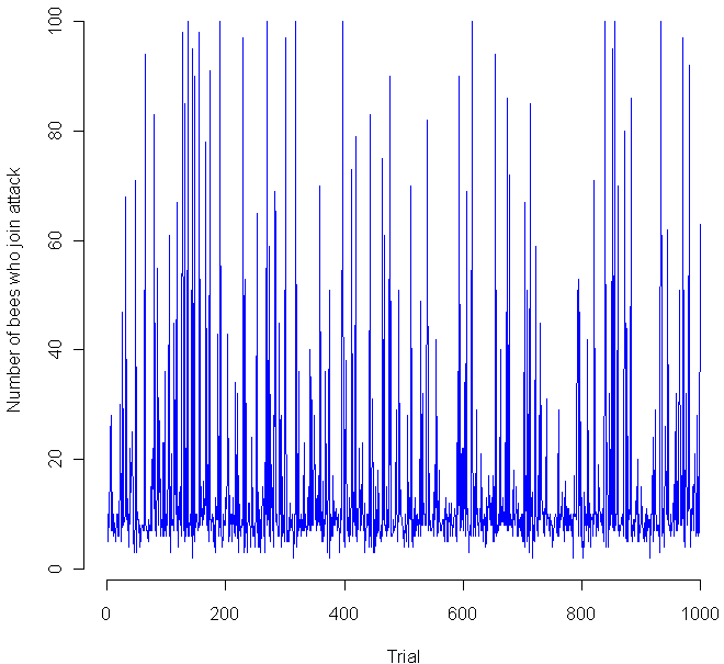
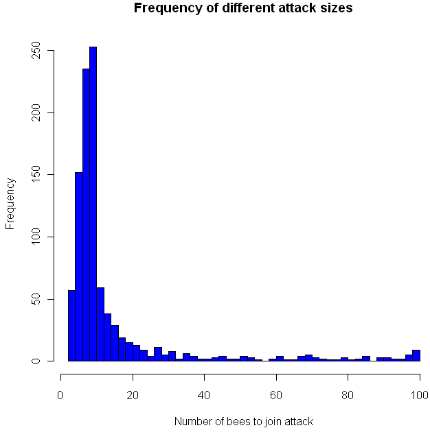
I think this last sentence is their way of noting that the exact distribution of sensitivities makes a huge difference in how the bees behave, which indeed it does. I decided to put the bees to the test, so I coded a simulation in the language R (code at the end of this post). I gave 100 virtual apis mellifera a random sensitivity level, chosen from a Uniform(1,100) distribution, then assumed 10 guards decided to attack. How would the others respond? Would a hair-trigger chain reaction occur? The chart at the top shows the results from 1000 trials. Looks pretty chaotic, so here’s a histogram of the results:

As you can see, most of the time the chain reaction dies out quickly, with no more than 20 new bees joining in the attack. However, occasionally the bees do go nuts, sending the full on attack. This happened about 1 percent of the time. Perhaps most interestingly, all of the other attack levels were clearly possible as well, in the flat zone from about 30 to 95. You might want to try playing with the distribution of the sensitivities and see if you get any other interesting distributions. Meanwhile, if you decide to raid a hive, make sure to dip yourself in mud first, that way the bees will think you are nothing but an innocent black rain cloud.

Code in R:

trials = 1000

go = rep(0,trials)
initial = 10

for(i in 1:trials) {
  bees = sort(runif(100,1,100))
  
  # Everyone who's threshold is less than the inital amount goes.
  going = length(bees[bees initial) {
    more = length(bees[bees going) {
    # Keep doing this until it stops
      going = more
      more = length(bees[bees