stats


20
Dec 11

Candidate Match Game


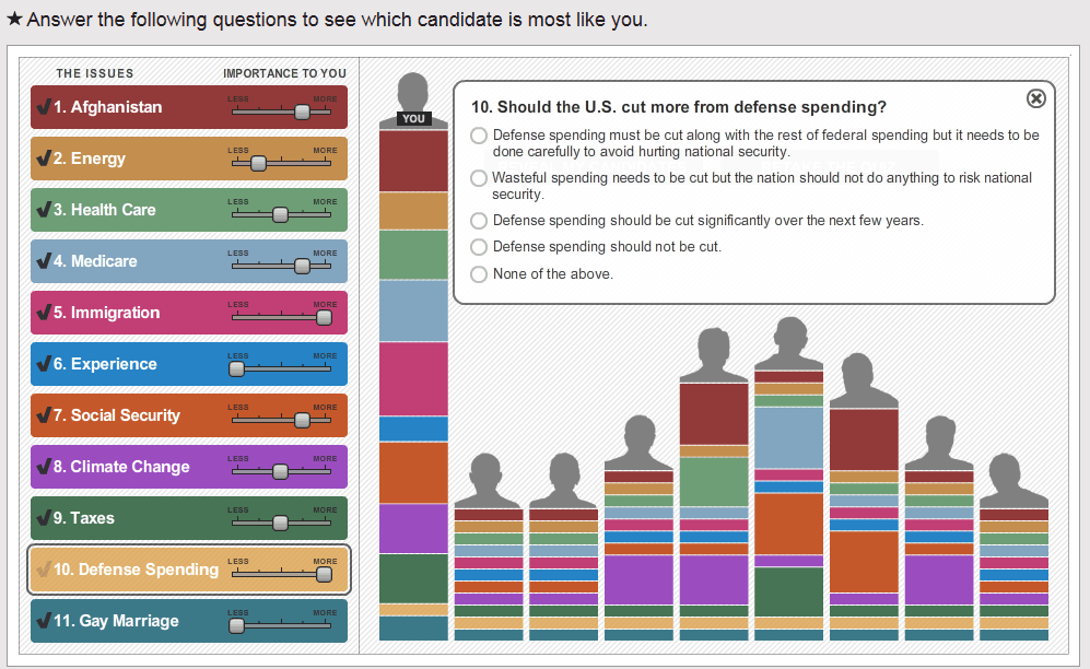
USA Today has an interesting quiz you can take that will match you up with a GOP presidential candidate. It’s here.

I didn’t find the particular questions and answers satisfying, but I imagine they’ve tried to match these up as closely as possible with the candidates’ positions. There are some interesting features to the quiz. For starters, it’s a nice piece of information architecture. The colors make it easy to track how each answer is reflected in each of the candidates’ rankings. The sliders, which let you set importance of the issues, are fun to use, and you can adjust any one of them at any time, so you can see how varying your weights effects each candidates’ score. I like that it also shows candidate “you”: this gives a feel for how closely you match up with the candidates in general. The closer the top candidate is to your bar, the closer the fit. Another nice touch: the way that the candidates are obscured by only showing silhouettes until you are done filling out the quiz. I would imagine this makes it less likely that you will try and tweak your answers and weightings to favor your favorite candidate, though if you look closely enough you can make out at least a couple of the candidates just from their silhouettes.

One final interesting note. The weightings are linear and additive. Another way to do the quiz might be to find the candidate with the best weighted geometric average. Depending on how the sliders were done, this could give you a “kill switch” to eliminate candidates who took a position opposite from yours on a single, vital issue (ie abortion). On the other hand, I suppose if you are a single issue voter you already know how each of the candidates stand on that issue.


6
Dec 11

My oh my

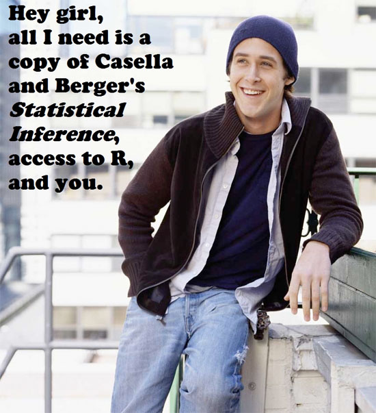
Noted without comment, visit Biostatistics Ryan Gosling !!! for more gems like the one above.


3
Dec 11

The first thing you learned about probability is wrong*


*or dangerously incomplete.

I’ve just started reading Against the Gods: The remarkable Story of Risk, a book by Peter Bernstein that’s been high on my “To Read” list for a while. I suspect it will be quite interesting, though it’s clearly targeted at a general audience with no technical background. In Chapter 1 Bernstein makes the distinction between games which require some skill, and games of pure chance. Of the latter, Bernstein notes:

“The last sequence of throws of the dice conveys absolutely no information about what the next throw will bring. Cards, coins, dice, and roulette wheels have no memory.”

This is, often, the very first lesson that gets presented in a book or a lecture on probability theory. And, so far as theory goes it’s correct. For that celestially perfect fair coin, the odds of getting heads remain forever fixed at 1 to 1, toss after platonic toss. The coin has no memory of its past history. As a general rule, however, to say that the last sequence tells you nothing about what the next throw will bring is dangerously inaccurate.

In the real world, there’s no such thing as a perfectly fair coin, die, or computer-generated random number. Ok, I see you growling at your computer screen. Yes, that’s a very obvious point to make. Yes, yes, we all know that our models aren’t perfect, but they are very close approximations and that’s good enough, right? Perhaps, but good enough is still wrong, and assuming that your theory will always match up with reality in a “good enough” way puts you on the express train to ruin, despair and sleepless nights.

Let’s make this a little more concrete. Suppose you have just tossed a coin 10 times, and 6 out of the ten times it came up heads. What is the probability you will get heads on the very next toss? If you had to guess, using just this information, you might guess 1/2, despite the empirical evidence that heads is more likely to come up.

Now suppose you flipped that same coin 10,000 times and it came up heads exactly 6,000 times. All of a sudden you have a lot more information, and that information tells you a much different story than the one about the coin being perfectly fair. Unless you are completely certain of your prior belief that the coin is perfectly fair, this new evidence should be strong enough to convince you that the coin is biased towards heads.

Of course, that doesn’t mean that the coin itself has memory! It’s simply that the more often you flip it, the more information you get. Let me rephrase that, every coin toss or dice roll tells you more about what’s likely to come up on the next toss. Even if the tosses converge to one-half heads and one-half tails, you now know with a high degree of certainty what before you had only assumed: the coin is fair.

The more you flip, the more you know! Go back up and reread Bernstein’s quote. If that’s the first thing you learned about probability theory, then instead of knowledge you we’re given a very nasty set of blinders. Astronomers spent century after long century trying to figure out how to fit their data with the incontrovertible fact that the earth was the center of the universe and all orbits were perfectly circular. If you have a prior belief that’s one-hundred-percent certain, be it about fair coins or the orbits of the planets, then no new data will change your opinion. Theory has blinded you to information. You’ve left the edifice of science and are now floating in the either of faith.


25
Nov 11

Interactive map of US road fatalities


Fantastic map which shows the location of every death on US roads from 2001 to 2009. Go take a look then come back and tell me….

What location did you zoom in on first, and why?


23
Nov 11

Monty Hall revisited

Chances are you’ve already heard about the Monty Hall problem. I wouldn’t be mentioning it at all, except that I keep reading descriptions of the problem that miss the absolutely critical point. For those who are new to the problem, here’s a summary:

Suppose you’re a contestant on a game show. The host, Monty Hall, shows you three numbered doors. Two of these doors hide goats, which you don’t want, and one of them hides a shiny new convertible, which you do. Pick the right door and you go home with the convertible, pick the wrong door and you get the goat (which I suspect they don’t even really give you). You make your best guess and choose a door. But before showing what’s behind it, Mr. Hall opens one of the other two doors to reveal a goat. “Now”, he asks, “do you want to stick with your original choice, or do you want to switch doors to the other one that hasn’t been opened yet?”

While you try desperately to remember the rules for conditional probability, the studio audience yells out suggestions and an attractive model smiles at you, making you wonder if you should ask if she comes with the car, but then you realize she probably gets that question all the time. Time is running out! Should you switch doors?

The correct decision, at least in terms of maximizing your chances of winning the car (but, alas, not the model), is to switch. IQ Test Grand Champion and writer Marilyn Vos Savant famously answered the question in one of her columns. Her answer, that you should switch, was widely controversial. The math behind the solution is surprisingly simple, though it rarely seems be presented in a simple way. Your first guess has a one-in-three chance of being right. That means your first guess has a two-in-three chance of being wrong. If your first guess was wrong, that means the car must be behind one of the other two doors. Since Monty just showed you the goat, the car must be behind the other door. Switch and you will get the car for sure. If you don’t switch, your chance of winning remains one-in-three. If you do switch, it jumps up to two-in-three. So ignore the studio audience and don’t get distracted by the model. Just call out the number of that other door!

But wait! Did you catch the missing assumptions needed to make this solution work? The big one, for me, is that Monty Hall will always follow the same procedure of opening up a door with a goat, regardless of what’s behind the door you picked. If you distrust Monty, you might suspect that he will only show you a goat when you’ve picked the car, in order to entice you to switch and loose the car. In that case you should stick with the door you have. Or perhaps Monty shows the goat more frequently when the car is picked first (but not all the time), in which case switching may or may not be the best strategy.

The part where I yell
The problem here is that the Monty Hall problem MAKES NO SENSE WITHOUT AN EXPLICIT PRIOR on Monty Hall’s behavior. Sorry for the yelling, but the point is too important to miss. In this case, the prior is your belief about the procedure Monty is using, and how strongly you hold that belief to be true. The notion of a “prior” might be difficult to explain to a general audience, but assuming a particular one without stating it directly is poisonous. The Monty Hall problem, like many others, can’t be turned into math without first assuming some kind of probability distribution for the inputs.

Usually, when one the distributions of an input isn’t specified, we tend to assume that every possible option has an equal chance of occurring; in other words that we have a uniform probability distribution. This makes sense for another hidden assumption in the problem — that either the game show contestant has made his first pick randomly, or that the prizes were placed behind doors randomly. Though even here I tend to agree with mathematical historian Byron Wall, who argues that our default assumption of a set of equally likely events is problematic. But in the case of the Monty Hall problem, there’s no uniform to even assume. The set of possible ways that Mr. Hall could decide to act is infinite and unknowable.

How does Hall pick between the goats?
Another hidden assumption is that Monty randomizes which door to reveal if the unpicked doors are both hiding goats. If he didn’t, and you knew for sure that Monty would always pick the door with the lower number if when he had a choice, then the math works out differently. Now, if you pick door number 1 and Monty shows you a goat behind door number 3, you know for sure car must be behind door number 2. Switching guarantees you a win! If you pick door number 1 and Monty opens door number 2, that could mean either a car or a goat is behind door number 3. To calculate your odds of winning by switching, you can use Bayes’ theorem to find the probability that a car is behind door number 3, given that Monty reveled a goat behind door 2.

Work out the math, and you should get one-half. In other words, if Monty shows you door number 2, and if he’s using the rule stated above, then switching doors gives you a one-half probability of winning, as does staying with the door you have. It doesn’t matter. No matter which door Monty reveals, switching your pick is never worse than not switching, and sometimes it’s better to switch. That means it’s what game theorists call a dominant strategy, one you would always want to employ. Even so, since Monty’s door revealing rules can change your odds of winning, this is another hidden assumption that should have been made explicit.

Back when goats were golden
When the Monty Hall problem was originally described to me, I assumed that Monty had chosen a door to reveal at random, and that this door just happened to contain a goat. Perhaps not the most reasonable assumption to make, but at the time I was still young enough to think that winning a goat might be cooler than winning some K-car convertible (hum… maybe I still believe that). At any rate, I didn’t have the skills to work out a solution under my assumptions back then, but doing it now takes just a little bit of work.

The probability that you will win after switching, given that Monty “accidentally” reveals a goat, is actually the sum of two other probabilities. The first probability, that you will win by switching if both of the other doors contain goats, is zero. The second is the probability that only one of the two others doors was hiding a goat, in which case you will win for sure, since we already assumed that Monty revealed a goat. Because we know that Monty picked a goat by accident, we gain no additional information about the door we picked or the alternative we might switch to. Each one is equally likely to have the car, so switch or not, our probability of winning is one-half.

If you find this explanation confusing, you might want to try Jeffrey Rosenthal’s explanation, which shows how to re-normalize probabilities of events within your target condition.

The Man Who Loved Only Bayes
After publishing her solution, Vos Savant was flooded with letters telling her she got it wrong. I suspect that many of those readers were ignorant of her assumptions, though Vos Savant says that most people fully understood the problem, and simply didn’t accept her solution. One of the few accounts to mention the importance of Monty Hall’s procedural rules, even though that part only comes after 8 pages of discussion, is in Paul Hoffman’s “The Man Who Loved Only Numbers”. To explain why so many people, many of them with advanced degrees, got it wrong, Hoffman quotes mathematician Andrew Vázsonyi:

“Physical scientists tend to believe in the idea that probability is attached to things. Take a coin. You know the probability of a head is one-half. Physical scientists seem to have the idea that the probability of one-half is fused with the coin. It’s a property. It’s a physical thing. But say I take that coin and toss it a hundred times and each time it comes up tails. You will say something is wrong. The coin is false. But the coin hasn’t changed. It’s the same coin that it was when I started to toss it. So why did I change my mind? Because my mind has been upgraded with information. This is the Bayesian view of probability. It took me much effort to understand that probability is a state of mind.”

I might view probability more in terms of degrees of (rational) belief, but the Vázsonyi quote highlights a key component missing in much of science: the direct recognition that you have a prior, and that this prior is a form of bias, very often baked right into the model you have chosen. There is no escape from this bias! The frequentest approach to probability is really just a special case within the world of Bayesian inference, where you have picked an uninformative (or minimally informative?) prior. But even here you have to model the prior. You have to know: how are we assuming that Monty Hall makes his decision about showing the contestant a goat? Is it based on some fixed probability regardless of which door the contestant picks? Does Monty consult the entrails of a chicken? As mentioned before, the world of possibilities is infinite, and no progress can be made in terms of our understanding until we delineate a space in which our prior beliefs will live. Only once we’ve done that, implicitly or (preferably!) explicitly, can we test out our beliefs, and update them based Monty Hall’s actions.

9
Nov 11

Manifesto update

I just got done tweaking some of the points in my Manifesto and added a new one about evidence. As before, the Manifesto is a work in progress; your feedback is welcome here since you can’t post comments to pages in WordPress.


20
Oct 11

Queueing up in R, continued

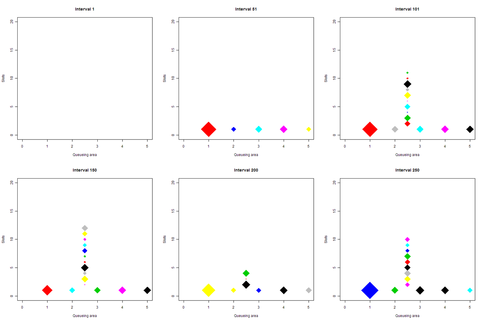
Shown above is a queueing simulation. Each diamond represents a person. The vertical line up is the queue; at the bottom are 5 slots where the people are attended to. The size of each diamond is proportional to the log of the time it will take them to be attended. Color is used to tell one person from another and doesn’t have any other meaning. Code for this simulation, written in R, is here. This is my second post about queueing simulation, you can find the first one, including an earlier version of the code, here. Thanks as always to commenters for their suggestions.

A few notes about the simulation:

  • Creating an animation to go along with your simulation can take a while to program (unless, perhaps, you are coding in Flash), and it may seem like an extra, unnecessary step. But you can often learn a lot just by “watching”, and animations can help you spot bugs in the code. I noticed that sometimes smaller diamonds hung around for much longer then I expected, which led me to track down a tricky little error in the code.
  • As usual, I’ve put all of the configuration options at the beginning of the code. Try experimenting with different numbers of intervals and tellers/slots, or change the mean service time.
  • If you want to run the code, you’ll need to have ImageMagick installed. If you are on a PC, make sure to include the full path to “convert”, since Windows has a built-in convert tool might take precedence. Also, note how the files that represent the individual animation cells are named. That’s so that they are added in the animation in the right order, naming them sequentially without zeros at the beginning failed.
  • I used Photoshop to interlace the animated GIF and resave. This reduced the file size by over 90%
  • The code is still a work in progress, it needs cleanup and I still have some questions I want to “ask” of the simulation.

13
Oct 11

Waiting in line, waiting on R

I should state right away that I know almost nothing about queuing theory. That’s one of the reasons I wanted to do some queuing simulations. Another reason: when I’m waiting in line at the bank, I tend to do mental calculations for how long it should take me to get served. I look at the number of tellers attending, pick an average teller session length (say one or two minutes), then come up with an average wait per person in line. For example, if there are 4 tellers and the average person takes 2 minutes to do her transaction, then new tellers should become available every 30 seconds. If I’m the 6th person in line, I should expect to wait 3 minutes before I’m attended.

However, based on my experience (the much maligned anecdotal), it often takes much longer than expected. My suspicion is that over time the teller’s get “clogged up” with the slowest people, so that even though an average person might take only 2 minutes, the people you actually see being attended right now are much more likely to be those who take a long time.

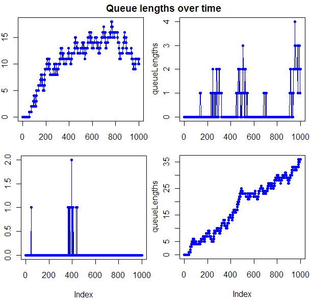
To explore this possibility, I set up a simulation in R (as usual, full source code provided at end of post). The first graph, at the beginning of this post, shows the length of queues over time for 4 runs of the simulator, all with the same configuration parameters. Often this graph was completely flat. Note though that when things get out of hand in terms of queue length, they can get way out of hand. To get a feel for how long you would have to wait, given that there is a line in front of you, I tracked how long the first person in line had to wait to be served. Given my configuration settings, this wait would be expected to last 5 intervals. It does seem to take longer than 5 intervals, though I want to tweak the model some and do more testing before I’m ready to quantify that wait.

There are, as with any models, things that make this one unrealistic. The biggest may be that people get in line with the same probability no matter how long the line is. What I need is some kind of tendency to abandon the line if it’s too long. That shouldn’t shorten the wait times for those already in line. I could make those worse. If you assume that slower people are prepared to wait longer in line, then the line is more likely to have slow people. Grandpa Jones is willing to spend an hour in line so he can chat for a while with the pretty young teller; but if the line is too long, that 50-year-old business guy will come back later to deposit his check. I would imagine that, from the bank’s perspective, this presents a tricky dilemma. The people whose time is worth the least are probably the most likely to be clogging up your tellers, upsetting the customers you care the most about (I know, I know, Bank of America cares about all of us equally, right?).

Code so far, note that run times can be very long for high intervals if the queue length gets long:

#### Code by Matt Asher. Published at StatisticsBlog.com ####
#### CONFIG ####
# Number of slots to fill
numbSlots = 5

# Total time to track
intervals = 1000

# Probability that a new person will show up during an interval
# Note, a maximum of one new person can show up during an interval
p = 0.1

# Average time each person takes at the teller, discretized exponential distribution assumed
# Times will be augmented by one, so that everyone takes at least 1 interval to serve
meanServiceTime = 25

#### INITIALIZATION ####
queueLengths = rep(0, intervals)
slots = rep(0, numbSlots)
waitTimes = c()
leavingTimes = c()
queue = list()
arrivalTimes = c()
frontOfLineWaits = c()


#### Libraries ####
# Use the proto library to treat people like objects in traditional oop
library("proto")

#### Functions ####
# R is missing a nice way to do ++, so we use this
inc <- function(x) {
  eval.parent(substitute(x <- x + 1))
}

# Main object, really a "proto" function
person <- proto(
	intervalArrived = 0,
	intervalAttended = NULL,
	
	# How much teller time will this person demand?
	intervalsNeeded = floor(rexp(1, 1/meanServiceTime)) + 1,
	intervalsWaited = 0,
	intervalsWaitedAtHeadOfQueue = 0,
)

#### Main loop ####
for(i in 1:intervals) {
	# Check if anyone is leaving the slots
	for(j in 1:numbSlots) {
		if(slots[j] == i) {
			# They are leaving the queue, slot to 0
			slots[j] = 0
			leavingTimes = c(leavingTimes, i)
		}
	}
	
	# See if a new person is to be added to the queue
	if(runif(1) < p) {
		newPerson = as.proto(person$as.list())
		newPerson$intervalArrived = i
		queue = c(queue, newPerson)
		arrivalTimes  = c(arrivalTimes, i)
	}
	
	# Can we place someone into a slot?
	for(j in 1:numbSlots) {
		# Is this slot free
		if(!slots[j]) {
			if(length(queue) > 0) {
				placedPerson = queue[[1]]
				slots[j] = i + placedPerson$intervalsNeeded
				waitTimes = c(waitTimes, placedPerson$intervalsWaited)
				# Only interested in these if person waited 1 or more intevals at front of line
				if(placedPerson$intervalsWaitedAtHeadOfQueue) {
					frontOfLineWaits = c(frontOfLineWaits, placedPerson$intervalsWaitedAtHeadOfQueue)
				}
				
				# Remove placed person from queue
				queue[[1]] = NULL
			}
		}
	}
	
	# Everyone left in the queue has now waited one more interval to be served
	if(length(queue)) {
		for(j in 1:length(queue)) {
			inc(queue[[j]]$intervalsWaited) # = queue[[j]]$intervalsWaited + 1
		}
		
		# The (possibley new) person at the front of the queue has had to wait there one more interval.
		inc(queue[[1]]$intervalsWaitedAtHeadOfQueue) # = queue[[1]]$intervalsWaitedAtHeadOfQueue + 1
	}
	
	# End of the interval, what is the state of things
	queueLengths[i] = length(queue);
}

#### Output ####
plot(queueLengths, type="o", col="blue", pch=20, main="Queue lengths over time", xlab="Interval", ylab="Queue length")
# plot(waitTimes, type="o", col="blue", pch=20, main="Wait times", xlab="Person", ylab="Wait time")

10
Oct 11

Drop in confidence

I’ve been paying a lot of attention lately to how statistics are released to the public. In particular, when are confidence intervals used, and when are they dropped? When are numbers presented as fact, and when are they acknowledged to be fuzzy?

The only time you consistently see confidence intervals reported, in the general press, is for poll results. As in: 66% of respondents believed this poll to be self-reflexive, with a margin of error of plus or minus 5%.

Weather reports often have percentages involved, but it would be a stretch to call these confidence intervals. For example, when the attractive meteorologist on Channel 7 tells you that there is an 80% chance of rain tomorrow, they are presenting that as a fact. Behind that number is a computer simulation that may or may not be able to estimate a confidence interval around that 80% number.

Government statistics and estimates, no matter how bad or biased, almost never come with confidence intervals attached. Gross Domestic Product of the U.S. in 2010? Estimated at $14.64 trillion. Confidence interval for that estimate? Probably so bad you don’t even want to know. Or maybe you do?

Are there times when you’ve been surprised to see a confidence interval reported or missing?


8
Feb 11

Power, p-values, publication bias and statistical evidence

I created this video to show as part of a presentation I’ll be giving next week. Your comments welcome, either here or at Youtube.