feature


25
May 10

How many tanks? MC testing the GTP

It’s 1943 and you work for the good guys. A handful of German tanks have been captured, and each one has a serial number. This is back when serial numbers were still presumed to come in serial, one right after the other. Given your collection of numbered tanks, and assuming that any existing tank was just as likely to be captured as any other, how many tanks would you guess that the Krauts have?

By luck, you have a time machine, so you jump forward in time, check out the Wikipedia entry, and copy down the formula [latex]\hat{N} = \frac{k+1}{k} m – 1 = m + \frac{m}{k} – 1[/latex], noting that [latex]m[/latex] should be replaced with the highest serial number encountered, while [latex]k[/latex] represents the number of tanks captured. Reading on, you see that Wikipedia has provided a rare nugget of actual understanding for a formula. This estimate represents “the sample maximum plus the average gap between observations in the sample”.

So you’re done, right? Just plug in to the formula, hand in your estimate to the commanding officer, go enjoy some R&R. Not so fast. Here at StatisticsBlog.com, nothing is believed to work until it passes the Monte Carlo test. To test out the formula I coded a simulation in R:

# Function to estimate maximum from sample "samp"
gTank <- function(samp) {
	 max(samp) + max(samp)/length(samp) - 1
}

# A blank log-log plot to get us started
plot(100,100, xlim=c(100,10^7), ylim=c(100,10^7), log="xy",pch=".",col="white",frame.plot=F,xlab="True value",ylab="Predicted")

# Let's track residuals
trueTops = c()
resids = c()
sampleTops = c()

x = runif(100,2,6)
for(i in x) {
	trueTop = 10^i
	for(j in 1:50) {
		observeds = sample(1:trueTop, 20) # No replacement here
		guess = gTank(observeds)

		# Plot the true value vs the predicted one
		points(trueTop,guess,pch=".",col="blue",cex=2) 

		trueTops = c(trueTops, trueTop)
		resids = c(resids, trueTop - guess)
		sampleTops = c(sampleTops, max(observeds))
	}
}

# Platonic line of perfectly placed predictions
lines(c(100,10^6),c(100,10^6),lty = "dashed",col="gray",lwd=1)

# Plot residuals too
windows()
plot(trueTops,log="x",resids,pch=20,col="blue",xlab="True value",ylab="Residual",main="Residuals plot")
abline(h=0)

mean(abs(resids))
mean(trueTops-sampleTops)

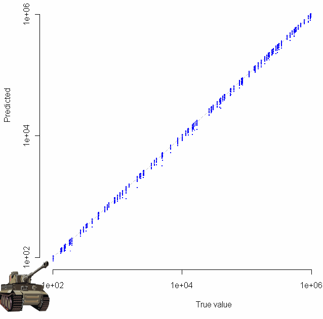
Which produces the following log-log plot:

Gratuitous clip art was added with the “chartJunk()” function.

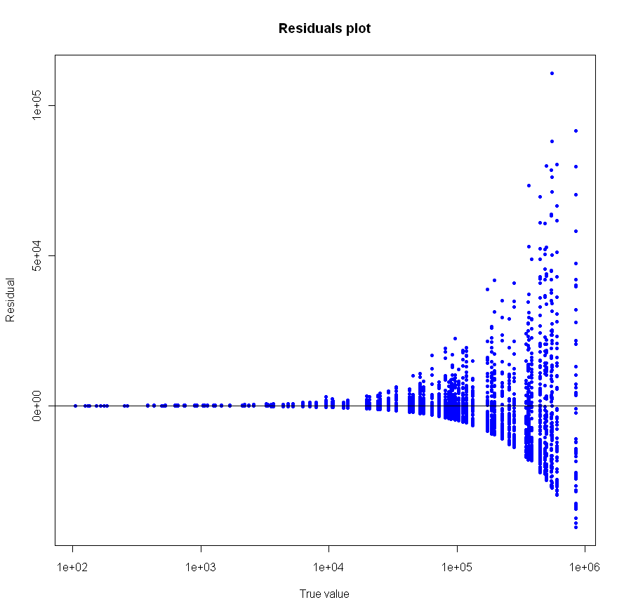
Looks pretty good, no? Especially given that the sample size for each of these tests was just 20. To make sure everything was OK, I plotted the residuals as well:

Make sure to click on the images above to see larger versions. Bigger really is better when it comes to viewing charts. Looks good too, no?

So, German tank problem estimate? Confirmed. Just don’t dig too deep into the assumption that all tanks had an equal chance of being captured; common sense goes against that one (ask yourself if there might be a relationship between length of time a tank is in the field of battle and the likelihood it will be captured).

Speaking of likelihood… this problem gives a nice example of how maximum likelihood estimation (MLE) can fail in spectacular form, like a bomb whose innards have been replaced by sawdust (alright, I promise, last military analogy). The MLE for the number of German tanks is the highest serial number observed. This is because MLE works backwards, finding the parameter which makes our observation most likely in terms of joint conditional probability. As a result, the MLE for this problem is not only biased (since it will always be less than or equal to the true number of tanks), but dumb as well. How likely is it (in the common sense usage of the term) that your captured tanks will include the highest-numbered one? If the distribution is truly uniform, the chance that you have to top one is [latex]\frac{k}N[/latex] where [latex]N[/latex] is the true, unknown number of tanks. You don’t know [latex]N[/latex], but you do know that it’s at least [latex]m[/latex] (the highest number observed). For small samples, where [latex]k << m[/latex], the probability that you have captured the very top-numbered tank is quite small indeed, no larger than [latex]\frac{k}m[/latex] at best.

Just how bad is the MLE? I compared the mean absolute residuals from the two different methods. Using the formula from at the beginning of this post gives 6,047. Using MLE, the average residual was 8,175, or 35% worse. Standard deviation for the MLE method is also higher, by about 27%. Back to boot camp for the MLE. (I know, I know, I promised).

20
May 10

R: A random walk though OOP land.

If you are used to object oriented programing in a different language, the way R does things can seem a little strange and backwards. “proto” to the rescue. With this library you can simulate “normal” OOP. I found the examples for proto not so helpful, so to figure out how the package works I sent one lonely red ant on a drunken walk. Here’s my code:

 
library("proto")

# Everybody likes ants
ant <- proto(
	# Default values for the class variables
	xPos = 0,            
	yPos = 0,
	name = character(),      
)

# What do ants do? They move
ant$move <-function(.,xDisp=0, yDisp=0) {
	.$xPos = .$xPos + xDisp
	.$yPos = .$yPos + yDisp
}

# See the little red ant move
ant$plot <- function(.) {
	points(.$xPos, .$yPos, pch=20, col="red")
}

# Instantiate the class. 
myAnt = ant
myAnt$name = "George"


plot(myAnt$xPos, myAnt$yPos, xlim=c(-10,10), ylim=c(-10,10), pch=20, col="red")
for(i in 1:40) {

	# The ant is drunk on Kool Aid
	myAnt$move(rnorm(1),rnorm(1))
	
	# The ant is lazy and will rest for a moment
	Sys.sleep(.5)
	
	# Plot the new location
	ant$plot()
	
}

cat("The ant named", myAnt$name, "is now located at (", myAnt$xPos, myAnt$yPos, ")\n")

18
May 10

R: Dueling normals

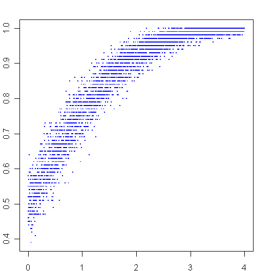
More playing around with R. To create the graph above, I sampled 100 times from two different normal distributions, then plotted the ratio of times that the first distribution beat the second one on the y-axis. The second distribution always had a mean of 0, the mean of first distribution went from 0 to 4, this is plotted on the x-axis.

Here is my code:

 
AbeatsB <- function(a,b) {
	sum(a>b)/length(a)
}

x = seq(0,4,.001)
y = c()
for (i in x) {
	y = c(y,AbeatsB(rnorm(100,i),rnorm(100,0)))
}

plot(x,y,pch=".",cex=2,col="blue")

12
May 10

Taking the “con” out of econometrics

Very interesting discussion between Ed Leamer and Russ Roberts about measuring statistical effects in the world of economics, and the often problematic desire to generalize conclusions. Here’s the link.


7
May 10

Connecting R and Python

There are a few ways to do this, but the only one that worked for me was to use Rserve and rconnect. In R, do this:

 
install.packages("Rserve")
library(Rserve)
Rserve(debug = FALSE, port=6311, args=NULL)

Then you can connect in Python very easily. Here is a test in Python:

 
rcmd = pyRserve.rconnect(host='localhost', port=6311)
print(rcmd('rnorm(100)'))

6
May 10

R: choose file dialog box

Needed this one recently, it pops up a window to pick a file to be used by r, then reads the contents into myData:

myFile <- file.choose()
myData  <- read.table(myFile,header=TRUE)

5
May 10

Game of Life in R

Before I decided to learn R in a serious way, I thought about learning Flash/Actionscript instead. Most of my work involves evolutionary models that take place over time. I need visual representations of change. It’s certainly possible to represent change and tell an evolving story with a single plot (see for example Tufte’s favorite infographic), but there are a lot more options when you can use animations. Flash is also object oriented, well documented with hundreds of books and websites, and has a powerful (albeit challenging to learn) IDE which helps for large coding projects.

The drawbacks to Flash are that it is way behind R in terms of statistical tools, is a closed, expensive language to work with, and dispute widespread use it might be so weak that a Apple’s iPhone might kill it.

So I picked R, with the idea that when I needed animations, I would find a way to build them. The code below is my first test of using R to generate animations. It’s a variant of Conway’s Game of Life (not to be confused with the Milton Bradley version), where single celled lifeforms live or die based on how many living neighbors they have. In my version, the rules for each cell are determined randomly, in advance of the game. The board size is fixed (see the configuration options at the beginning), whereas Conway’s version was played on a theoretically infinite grid. Green cells are “alive”, black ones are “dead”. I tried for nearly an hour to match the Black=living, White=dead scheme of Conway but couldn’t get that to work, maybe you can figure out how to do it. I re-sized the resulting animated GIF with an external program, that’s another thing I still need to figure out in R.

par(mar=c(0,0,0,0))
library(abind)
library(gdata)
library(fields)
library(grDevices)
library(caTools)
#
times = 50
myWidth = 10
myHeight = 10
#   
# Set the 3D array of rules to determine transitions for each cell.
rulesArray = NULL
for(i in 1:9) {
	toBind <- matrix(sample(c(0,1),replace=T,(myWidth*myHeight)),ncol=myWidth)
	rulesArray <- abind(rulesArray, toBind, along=3)
}
#
first = T
frames = array(0, c(myWidth, myHeight, times))
for(i in 1:times) {
	if(first) {
		forFrame <- sample(c(0,1),replace=T,(myWidth*myHeight))
		first = F
	} else {
		# Convert last frame data to matrix to make comparing adjacent cells easier
		forFrame <- matrix(forFrame, ncol=myWidth)
		newFrame <- forFrame
		#
		for(m in 1:myHeight) {
			for(n in 1:myWidth) {
				adjLiving = 1 # cuz we start with array index 1
				#
				# Find out how many adjacent are living
				if(m > 1 && n > 1) {
					# Look at top left
					adjLiving = adjLiving + forFrame[(m-1),(n-1)]
				}
				if(m > 1) {
					# Look at top center
					adjLiving = adjLiving + forFrame[(m-1),(n)]
				}
				if(m > 1 && n < myWidth) {
					# Look at top right
					adjLiving = adjLiving + forFrame[(m-1),(n+1)]
				}
				if(n > 1) {
					# Look at left
					adjLiving = adjLiving + forFrame[(m),(n-1)]
				}
				if(n < myWidth) {
					# Look at right
					adjLiving = adjLiving + forFrame[(m),(n+1)]
				}
				if(m < myHeight && n > 1) {
					# Look at bottom left
					adjLiving = adjLiving + forFrame[(m+1),(n-1)]
				}
				if(m < myHeight) {
					# Look at bottom center
					adjLiving = adjLiving + forFrame[(m+1),(n)]
				}
				if(m < myHeight && n < myWidth) {
					# Look at bottom right
					adjLiving = adjLiving + forFrame[(m+1),(n+1)]
				}
				#
				# Find the corresponding rule for this cell
				newStatus = rulesArray[m,n,adjLiving]
				#		
				# Update the status of this cell depending on the rule and number of living adjacent
				newFrame[m,n] = newStatus			
			}
		}
#		
		# Pull it out of a matrix
		forFrame = unmatrix(newFrame)	
	}
	frames[,,i] <- forFrame
}
write.gif(frames, "gameOfLifeRevisited.gif", col=c("#FFFF00", "#000000") , delay=150)

4
May 10

R: directing output to file on the fly, output flushing

To start sending all output to a file, do this:

sink("path/to/filename") # Direct all output to file
print("Hi there") # Will be printed to file
sink() # Turn off buffing to file

Related to this I recently had to use:

flush.console()

This forces your console to print out any buffered content. Doing this will cost time, but if you are running a very long script and wonder if it is still alive, you might do something like this:

for(i in 10000:20000) { 
	# Find the i'th prime number
	# Are we still alive?
	cat("."); flush.console()
}

3
May 10

First annual R plot replication prize

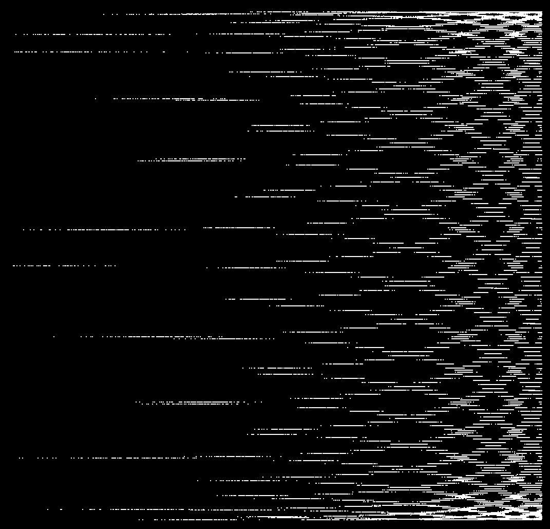
Click image for the full-size version

$100 to the first person who can figure out how I created this plot and replicate it. Some hints:

  • It was done in R.
  • There is only one underlying probability distribution involved (one “rdist()“).
  • Including the “plot” statement, I created this with 3 short lines of code.

This is based on a random sampling of unstated size, so I don’t expect that your graph will be an absolute, exact match.

I’ll add $1 to the prize for every day that goes by without a winner until the end of the year. After that I’ll consider it an unsolved mystery and reveal the code I used.

Post your guesses for the code as a comment to this post. First correct answer wins. Good luck to all!


2
May 10

Anthropic principle visited (because I can visit it)

The Anthropic Principle justifies the existence of life against apparently infinitesimal small scientific odds of a life-sustaining universe. The arguments behind it can be fairly complex, but I think the most important part can be summed up very easily:

“If the outcome had been negative, we wouldn’t be around to witness it.”

In other words, if the universe had been inhospitable to human life, no one would be around to verify what came to pass. Although it is usually limited to justifying life on earth, the anthropic principle goes well beyond the cosmological. It effects how we understand any rare event which happens to happen to us.

Start with an extreme event. A fully loaded bus slides over the guardrail on a mountain pass. Ninety nine passengers die. One survives. It would hardly be surprising if that one passenger says God, and not random luck, saved her. After all, she alone survived, miraculously, while everyone else perished in a wreck which seemed destined to kill everyone.

But how do the other 99 passengers feel? Did God choose them to die, just like He apparently choose her to live? Maybe we could interview them. Oh, wait.

Take thousands of individual events, each one extraordinarily improbable, and try them out with billions of people over and over. The most likely result, the most scientifically probable, is that some people will experience extremely unlikely occurrences. If they go on to ascribe those experiences to more than just blind luck that shouldn’t surprise us. It’s only natural. But it most certainly doesn’t prove divine intervention.

Think of it this way: You, the consciousness reading these very words, are the product of millions of little events which could have just as easily gone the other way: If you mother didn’t have a soft spot for men with mustaches, if you great-grandfather hadn’t been shot down over France, if you great-great grandfather hadn’t bumped his head on that giant bottle of Sam’s Cure-all Tonic, you won’t be here today. You’re as unlikely as a tossed coin landing on its side. The universal probability bound is broken every day.

Of course the same thing goes for everyone else around you. Ten billion souls, each one coming into existence despite near impossible odds. Ten billion miracles, right? Only if you discount the stega-godzillion souls who’s coin flips landed the usual way and were never born. They are mute, silent, YouTube-impaired, invisible non-witnesses to their own bell-curve filling banality.