art


15
Mar 16

Probability Podcast Ep2: Imprecise probabilities with Gert de Cooman

Gert

I happened to be travelling through Brussels, so I stopped by Ghent, the world hotspot for research into imprecise probabilities, and setup an interview with Gert de Cooman. Gert has been working in imprecise probabilities for more than twenty years, is a founding member and former President of SIPTA, the Society for Imprecise Probability: Theories and Applications, and has helped organize many of the ISIPTA conferences and SIPTA Schools.

Topics include fair betting rates, Dutch books, Monte Carlo methods, Markov chains, utility, and the foundations of probability theory. We had a rich, wide-ranging discussion. You may need to listen two (or more!) times to process everything.


Episode on SoundCloud


12
Jun 14

A new way to visualize content

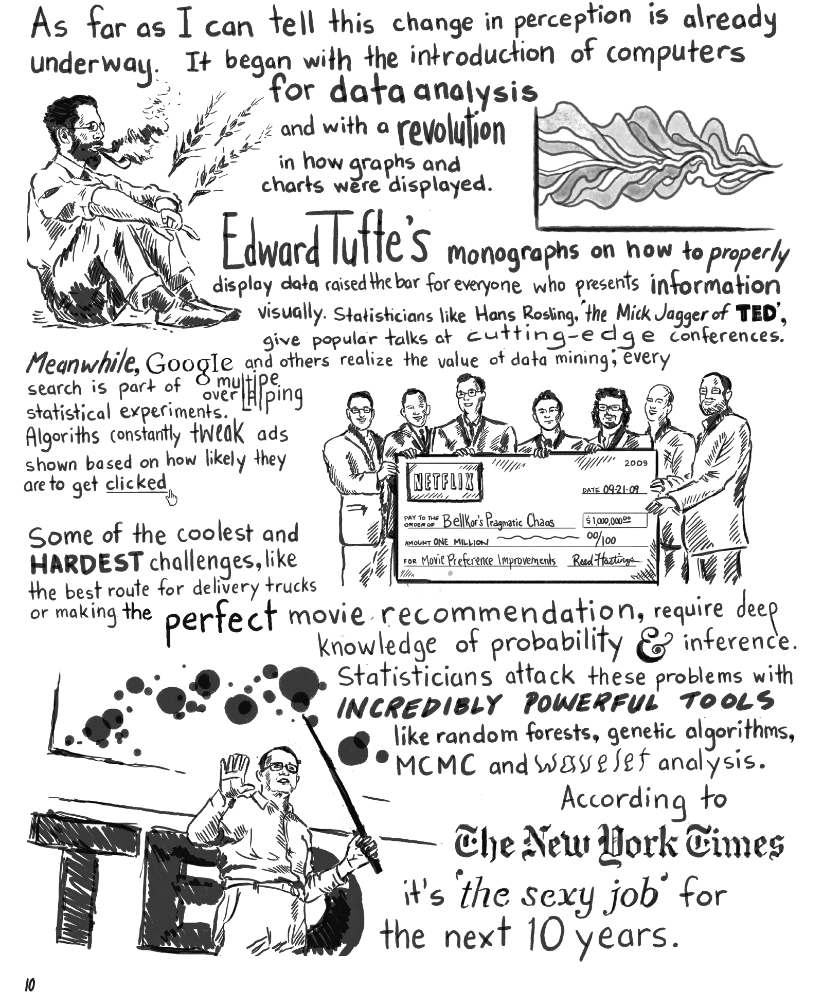
Right now I’m working on a project that involves new ways to view units of content and the relationships between them. I’ve posted the comic I worked on, it has a number of stats references throughout. This is early alpha stages for the software, you may run into issues. To see the relationships, go to the puffball menu and make sure that “Show relationships” is clicked.


14
Feb 13

Population simulation leads to Valentine’s Day a[R]t

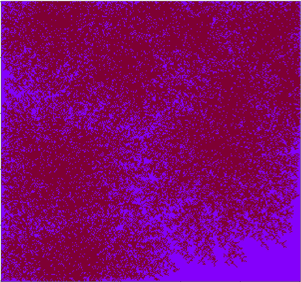
Working on a quick-and-dirty simulation of people wandering around until they find neighbors, then settling down. After playing with the coloring a bit I arrived at the above image, which I quite like. Code below:

# Code by Matt Asher for statisticsblog.com
# Feel free to modify and redistribute, but please keep this notice 

maxSettlers = 150000

# Size of the area
areaW = 300
areaH = 300

# How many small movements will they make to find a neighbor
maxSteps = 200

# Homesteaders, they don't care about finding a neighbor
numbHomesteaders = 10

areaMatrix = matrix(0, nrow=areaW, ncol=areaH)

# For the walk part
adjacents = array(c(1,0,1,1,0,1,-1,1,-1,0,-1,-1,0,-1,1,-1), dim=c(2,8))

# Is an adjacent cell occupied?
hasNeighbor <- function(m,n,theMatrix) {
	toReturn = FALSE
	for(k in 1:8) {
		yCheck = m + adjacents[,k][1]
		xCheck = n + adjacents[,k][2]
		if( !((xCheck > areaW) | (xCheck < 1) | (yCheck > areaH) | (yCheck < 1)) ) {
			if(theMatrix[yCheck,xCheck]>0) {
				toReturn = TRUE
			}
		}
	}
	return(toReturn)
}


# Main loop
for(i in 1:maxSettlers) {
	steps = 1
	xPos = sample(1:areaW, 1)
	yPos = sample(1:areaH, 1)
	
	if(i <= numbHomesteaders) {
		# Seed it with homesteaders
		areaMatrix[xPos,yPos] = 1
	} else {
		if(areaMatrix[xPos,yPos]==0 & hasNeighbor(xPos,yPos,areaMatrix)) {
			areaMatrix[xPos,yPos] = 1
		} else {
			spotFound = FALSE
			outOfBounds = FALSE
			
			while(!spotFound & !outOfBounds & (steps areaW) | (xPos < 1) | (yPos > areaH) | (yPos < 1)) {
					outOfBounds = TRUE
				} else if(hasNeighbor(xPos,yPos,areaMatrix) ) {
					areaMatrix[xPos,yPos] = steps
					spotFound = TRUE
				}
			}
		}
		
	}

}
	
image(areaMatrix, col=rev(rgb(seq(0.01,1,0.01),seq(0.01,1,0.01),seq(0.01,1,0.01))))

# I think this version looks nicer!
# areaMatrix[areaMatrix !=0] = 1
# image(areaMatrix, col=rev(rgb(.5,0,seq(0.2,1,0.2))))

14
Dec 12

Let it snow!

A couple days ago I noticed a fun piece of R code by Allan Roberts, which lets you create a digital snowflake by cutting out virtual triangles. Go give it a try. Roberts inspired me to create a whole night sky of snowflakes. I tried to make the snowfall look as organic as possible. There are lots of options to adjust. Here’s the code, have fun and Happy Holidays!

# Code by Matt Asher for statisticsblog.com
# Feel free to modify and redistribute 

# How many flakes do you want to fall?
flakes = 100

# Width and height of your space
width = 800
height = 600

# Initial wind
wind = 0

# Setup the background of the plot and margins
par(bg = "black")
par(oma=c(0,0,0,0))
par(mar=c(0,0,0,0))
plot(0, 0, col="black", pch=".", xlim=c(0,width), ylim=c(0,height), axes=F)

for(i in 1:flakes) {
    startY = height
    startX = runif(1,1,width)

    xPos = startX
    yPos = startY

    for(j in 1:height) {

		# Optional drift in wind
		wind = wind + rcauchy(1,0,.05)

		# Update snowflake position
        xPos = xPos + rnorm(1,.1,1.5)
        yPos = yPos - runif(1,4,20)

        # Are we in the space, if so display it
        if(xPos > 0 && xPos <= width && yPos > 0 && yPos <= height) {
            points(round(xPos), round(yPos), col="white", pch=8)

            # System dely, slows down the flakes
            Sys.sleep(0.1)
        }
    }
}

23
Oct 12

Comic with stats discussion

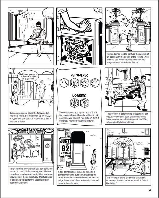
I recently finished work on the first issue of a graphic novel. It’s in the form of a fictional first person narrative. The story isn’t directly about statistics, but there are a few digressions on the subject. Here are some samples, make sure to click on the images for a larger view:

If you’re interested, head over to sunfalls.com and pick up a copy. Here’s the order page. The comic comes with a full money-back guarantee, including shipping. You don’t even have to send back your copy to claim the refund.


15
Jan 12

R A Fisher illustration


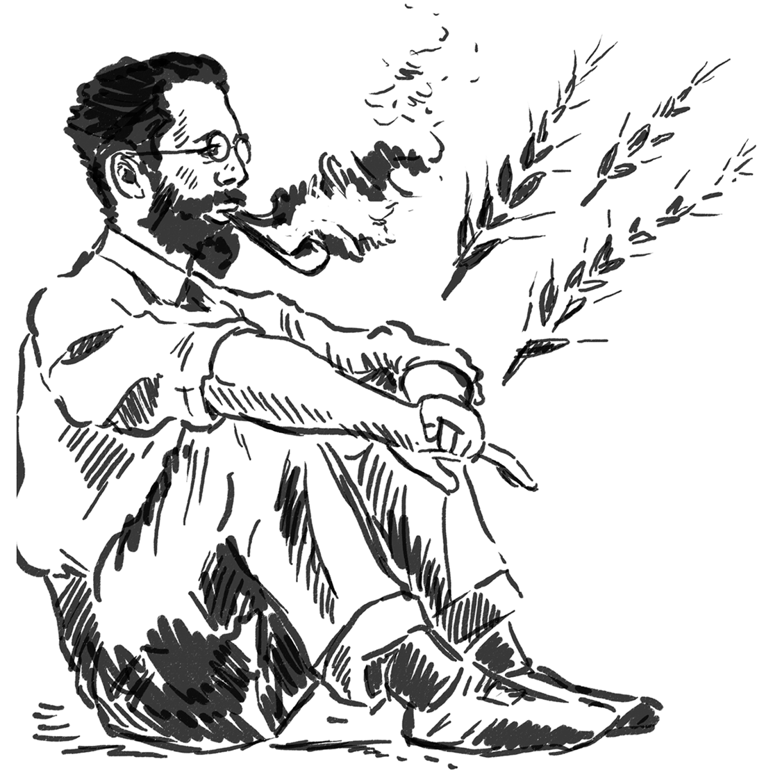
Ronald Aylmer Fisher, statistics badass. Illustration by Rachelle Scarfó for a project I was working on.


4
Sep 10

Weekend art in R (Part 4)

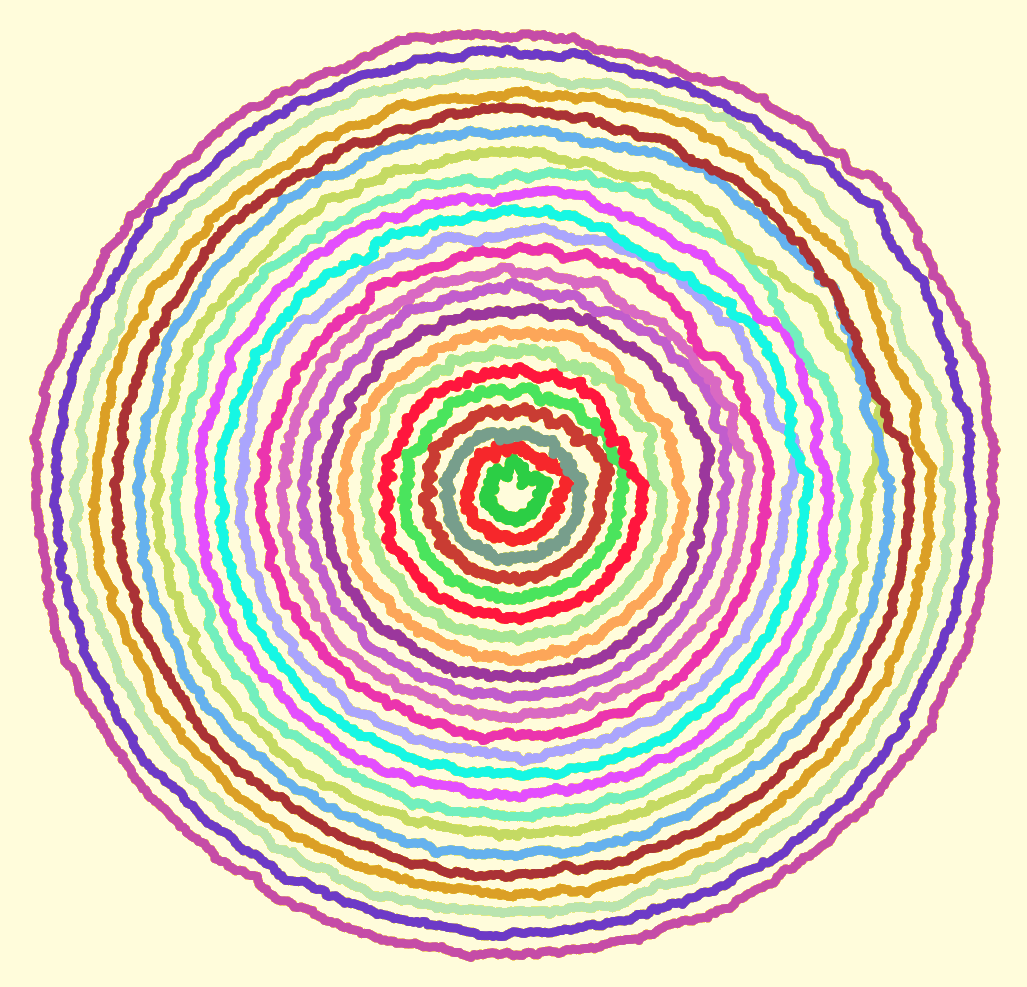
Computer creations are perfect by design. We put in numbers, and if all goes well we get out an exact result. If we want a line, we want it perfectly straight. If we want a circle, it should conform to the platonic ideal of a circle. From a mathematical standpoint, these perfect shapes and precisely computed numbers are ideal.

Someday, perhaps, we will have true fuzzy computation built right into our hardware. For now, it takes considerable effort to achieve just the right level of imperfection needed for simulating mistakes, or any organic processes.

I sent each of the circles shown above on a random walk. That part was easy, getting each circle to end up where it started (and close the loop) took a bit more effort. To vary the “wigglyness” of the lines, adjust the “sd” parameter in “rnorm”. To change how quickly randomness tapers off, change the “4” in “i/4”. Here is my code:

# Circle lengths
j = seq(0.1,1.9,.08)

par(bg = "black")
plot(-2,-2,pch=".",xlim=c(-2,2),ylim=c(-2,2),col="white")

# How many dots around the circle?
dots = 1000

# Create an offkilter circle
rads = seq(0,2*pi,2*pi/dots)

for(aLength in j) {
	# Pick a random color
	myCol = paste("#",paste(sample(c(1:9,"A","B","C","D","E","F"),6,replace=T),collapse=""),collapse="",sep="")
	
	# Start at length = 1, then walk.
	myLength = rep(aLength,dots)
	
	for(i in 2:dots) {
		myLength[i] = myLength[(i-1)] + rnorm(1,0,sd=.005)
		
		# Closer we are to end, faster we return to where started so circle closes
		dist = aLength - myLength[i]
		myLength[i] = aLength - (dist*((dots-(i/4))/(dots)))
	}


	for(i in 1:dots) {
		cat(myLength[i]*cos(rads[i]),myLength[i]*sin(rads[i]),"\n")
		points(myLength[i]*cos(rads[i]),myLength[i]*sin(rads[i]),col=myCol,pch=20,cex=2)
	}
}
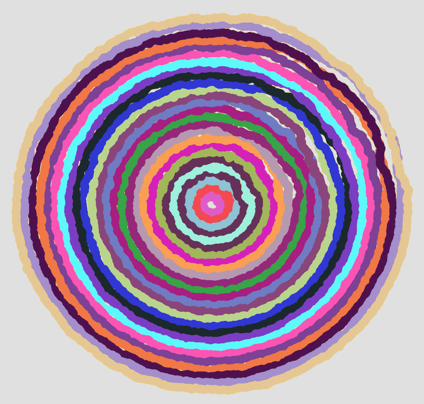
What do your circles look like?


21
Aug 10

Weekend art in R (Part 3)

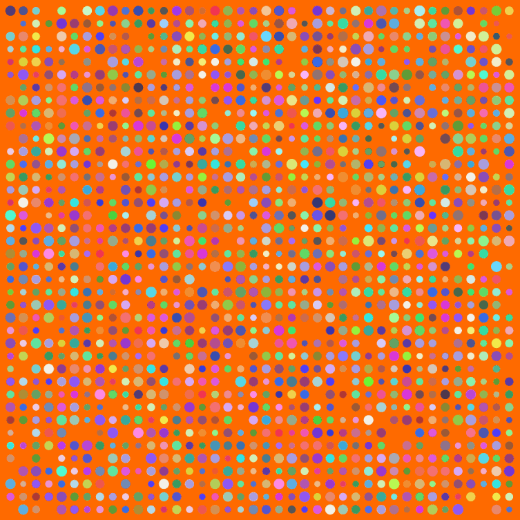
I have a few posts nearing completion, but meanwhile a weekend break for art. Big thanks to Simon Urbanek and Jeffrey Horner, creators of Cairo, a library for the programming language R. Have you noticed how R can’t anti-alias (fancy way for saying smooth out lines and curves when creating a bit-mapped image)? Cairo can.

Make sure to click the image above for the full version. Here’s my code:

# The Cairo library produces nice, smooth graphics
Cairo(1200, 1200, file="D:/Your/Path/Here/Dots.png", type="png", bg="#FF6A00")

# How big should the grid for placing dots be?
myWidth=40
myHeight=40

dotsPlaced = myWidth*myHeight

# Optional default colors and sizes for dots
myColors = rep(c("#0000F0","#00F000"),dotsPlaced)
myCex = rep(3.2,dotsPlaced)

for(i in 1:dotsPlaced) {
	# Change this to allow more of the default color dots to survive
	if(runif(1)<1) {
		myColors[i] = paste("#",paste(sample(c(3:9,"A","B","C","D","E","F"),6,replace=T),collapse=""),collapse="",sep="")
	}
	myCex[i] = runif(1,3,6)
}

# Keeping this is marginal
par(oma=c(0,0,0,0))
par(mar=c(0,0,0,0))

# Start off with a blank plot. The white dot helps with cropping later
plot(0,0,pch=".",xlim=c(0,40),ylim=c(0,40),col="white", xaxt = "n", yaxt = "n")

for(m in 1:myWidth) {
	for(n in 1:myHeight) {
		if(runif(1) < .93) {
			points(n,m,pch=20,col=myColors[((m*n)+n)],cex=myCex[((m*n)+n)])
		}
	}
}

dev.off() # Tell Cairo to burn the plot to disk

10
Jul 10

Photo without caption


26
Jun 10

Weekend art in R (Part 2)

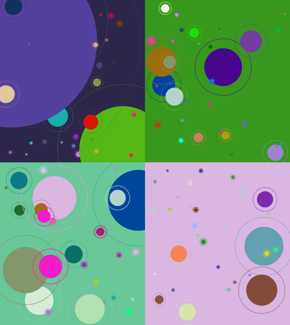
I put together four of the best looking images generated by the code shown here:

# More aRt
par(bg="white")
par(mar=c(0,0,0,0))
plot(c(0,1),c(0,1),col="white",pch=".",xlim=c(0,1),ylim=c(0,1))
iters = 500
for(i in 1:iters) {
	center = runif(2)
	size = 1/rbeta(2,1,3)
 
	# Let's create random HTML-style colors
	color = sample(c(0:9,"A","B","C","D","E","F"),12,replace=T)
	fill = paste("#", paste(color[1:6],collapse=""),sep="")
	brdr = paste("#", paste(color[7:12],collapse=""),sep="")
 
	points(center[1], center[2], col=fill, pch=20, cex=size)
	points(center[1], center[2], col=fill, pch=21, cex=size,lwd=runif(1,1,4))
}

Weekend art Part 1 is here.