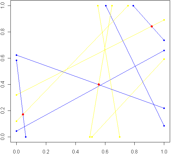
Imagine a unit square. Every side has length 1, perfectly square. Now imagine this square was really a fence, and you picked two spots at random along the fence, with uniform probability over the length of the fence. At each of these two locations, set down a special kind of cannon. Just like the light cycles from Tron, these cannons leave trails of color. To aim each cannon, pick another random point from one of the three other sides of the fence, and aim for that point.
Sometimes there will be a collision within the square, other times no. The image at top shows the results of five trials. The red dots are where the trails from a pair of cannons collided. My burning question: What is the distribution for these dots? Before reading on, try to make a guess. Where will collisions be most likely to happen?
Somewhere in the world, there lives a probabilist who could come up with a formula for the exact distribution in an hour, but that person doesn’t live in my house, so I took the Monte Carlo approach, coded in R:
# Functions to pick two points, not on the same side:
m2pt <- function(m) {
	if(m <1) {
		myPoint = c(5,m,0)
	} else if (m < 2) {
		myPoint = c(6,1,m %% 1)
	} else if (m < 3) {
		myPoint = c(7,1-(m %% 1),1)
	} else {
		myPoint = c(8,0,1-(m %% 1))
	}
	return(myPoint)
}

get2pts <- function() {
	pt1 = m2pt(runif(1,0,4))
	pt2 = m2pt(runif(1,0,4))

	# Make sure not both on the same sides. If so, keep trying
	while(pt1[1] == pt2[1]) {
		pt2 = m2pt(runif(1,0,4))
	}
	return(c(pt1[2:3],pt2[2:3]))
}

# Optional plot of every cannon fire line. Not a good idea for "iters" more than 100
#windows()
#plot(0,0,xlim=c(0,1),ylim=c(0,1),col="white")

# How many times to run the experiment
iters = 10000

# Track where the intersections occur
interx = c()
intery = c()

for(i in 1:iters) {
	can1 = get2pts()
	can2 = get2pts()

	# Optional plot of every cannon fire line. Not a good idea for "iters" more than 100
	#points(c(can1[1],can1[3]),c(can1[2],can1[4]),pch=20,col="yellow")
	#segments(can1[1],can1[2],can1[3],can1[4],pch=20,col="yellow",lwd=1.5)
	#points(c(can2[1],can2[3]),c(can2[2],can2[4]),pch=20,col="blue")
	#segments(can2[1],can2[2],can2[3],can2[4],pch=20,col="blue",lwd=1.5)

	# See if there is a point of intersection, find it.
	toSolve = matrix(c( can1[3]-can1[1], can2[3]-can2[1], can1[4]-can1[2], can2[4]-can2[2]),byrow=T,ncol=2)
	paras = solve(toSolve, c( can2[1]-can1[1], can2[2]-can1[2]))

	solution = c(can1[1] + paras[1]*(can1[3]-can1[1]), can1[2] + paras[1]*(can1[4]-can1[2]))

	# Was the collision in the square
	if(min(solution) > 0 && max(solution) < 1) {
		# Optional plot of red dots
		# points(solution[1],solution[2],pch=20,col="red",cex=1.5)

		# if this intersection is in square, plot it, add it to list of intersections
		interx = c(interx, solution[1])
		intery = c(intery, solution[2])
	}
}

windows()
plot(interx, intery, pch=20,col="blue",xlim=c(0,1),ylim=c(0,1))
After carefully writing and debugging much more code than I expected, I ran a trial with several thousand cannon fires and plotted just the collisions. Here is what I saw:
Looks pretty uniform, doesn't it? If it is, I will have gone a very long way just to replicate the bi-variate uniform distribution. My own original guess was that most collisions, if they happened in the square, would be towards the middle. Clearly this wasn't the case. Looks can be deceiving, though, so I checked a histogram of the x's (no need to check the y's, by symmetry they have the same distribution):
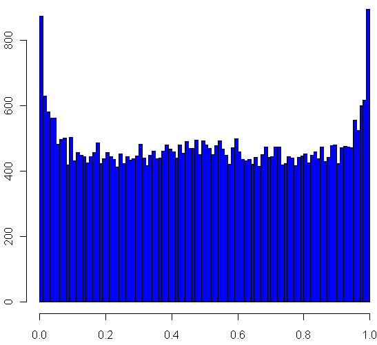
Very interesting, no? The area near the edges appears more likely to have a collision, with an overall rounded bowl shape to the curve. The great thing about Monte Carlo simulations is that if something unexpected happens, you can always run it again with more trials. Here I changed "iters" to 100,000, ran the code again, and plotted the histogram.
hist(interx, breaks=100, col="blue",xlab="x",main="Histogram of the x's")
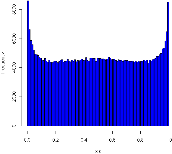
Now its clear that the distribution spikes way up near the edges, and appears to be essentially flat for most of the middle area. It seems like it may even go up slightly at the very middle. Just to be sure, I ran a trial with one million iterations:
Now it definitely looks like a small upward bulge in the middle, though to be sure I would have to do run some statistical tests or use an even larger Monte Carlo sample, and given how inefficient my code is, that could take the better part of a week to run. So for today I'll leave it at that.
One final statistic of note: During my run of one million iterations, 47.22% of all collisions happened inside the box. What do you think, is the true, theoretical ratio of collisions within the box a rational number?


