Posts Tagged: probability


15
Oct 15

Random samples in JS using R functions

For a JavaScript-based project I’m working on, I need to be able to sample from a variety of probability distributions. There are ways to call R from JavaScript, but they depend on the server running R. I can’t depend on that. I need a pure JS solution.

I found a handful of JS libraries that support sampling from distributions, but nothing that lets me use the R syntax I know and (mostly) love. Even more importantly, I would have to trust the quality of the sampling functions, or carefully read through each one and tweak as needed. So I decided to create my own JS library that:

  • Conforms to R function names and parameters – e.g. rnorm(50, 0, 1)
  • Uses the best entropy available to simulate randomness
  • Includes some non-standard distributions that I’ve been using (more on this below)

I’ve made this library public at Github and npm.

Not a JS developer? Just want to play with the library? I’ve setup a test page here.

Please keep in mind that this library is still in its infancy. I’d highly recommend you do your own testing on the output of any distribution you use. And of course let me know if you notice any issues.

In terms of additional distributions, these are marked “experimental” in the source code. They include the unreliable friend and its discrete cousin the FML, a frighteningly thick-tailed distribution I’ve been using to model processes that may never terminate.


1
Jul 13

Morality needs probability, manifesto addendum

Just added to my Big Bright Green Manifesto Machine. You might need to read this through a couple times; it’s a difficult concept since it lives in a collective blind spot for us:

Doing ethics without probability is like performing surgery with a wooden spoon — it’s a blunt instrument capable of only the most basic operations, and more likely to kill the patient than heal them. Implicitly, we understand this need for probability in making ethical judgements, yet most people recoil when the calculus of probabilities is made explicit, because it seems cold, because the math frightens and confuses them, or because letting odds remain unestimated and unacknowledged allows people to confuse positive outcomes with moral behavior, sweeping hidden risks under the rug when things go well, or claiming ignorance when they don’t. It’s time to acknowledge — directly, explicitly, mathematically — that morality needs probability. For ethics to move forward it must be integrated with our knowledge of randomness and partial entailment.

Here’s an example of how we already take probability into account implicitly. If we retrieve our lost ball from someone’s yard without asking first, we justify this based on our belief that the owner is more likely to be bothered by us interrupting their dinner, than by our temporary trespass on their lawn. The greater the probability of great harm, the higher the level of certainty we demand. Our most heated debates involve situations where the probability of harm from both action and inaction is high. If someone’s dog is stuck in a hot car on a sunny day, should you break in and try to save it? Does the chance of a dog dying of heatstroke justify a forced entry that will probably result in expensive damage and an irate owner (though it’s possible they would be grateful instead). If you decide to break in, how long should you wait first? What prior distribution should you put on the owner’s return time, and how do you update your prior as time goes by? If the waiting time is chi-square on low degrees of freedom, your concern for the dog might be unjustified. If it follows the unreliable friend distribution, you may be that dog’s only hope.

As I hope is becoming clear, questions of morality cannot be resolved without asking questions about probability. If the example above seems trivial (perhaps the owner’s property rights trump your concern for a dog), then substitute the animal for a toddler who looks uncomfortably warm. Now how long do you wait, and how do you deal with the risk that smashing a window might harm the child?


23
Feb 12

A classification scheme for types of randomness

We often speak implicitly of different types of randomness but neglect to name or categorize them. Consider this post to be a kind of white paper or rough draft on the division of randomness into five categories. If you start using these distinctions explicitly, even if only in your own head, I think you will find them highly useful, as I have.

Type 0: Fixed numbers or known outcomes

Type 0 randomness is the special case of randomness where the data are already known. Any known outcome, regardless of the process that generated it, is Type 0 randomness. Once known, it has become a constant. In terms of information conveyed, all Type 0 randomness has zero informational entropy (a measure of uncertainty), and all messages with zero entropy are examples of Type 0 randomness.

Type 1: Pseudo random.

Most computers generate random numbers by a deterministic process. An initial “seed” is picked using some environmental factor, like the microsecond timing of the CPU, and from there onward every number that follows is fully determined by the algorithm. These algorithms can be very good, in terms of producing sequences of numbers that have desirable qualities. Yet, if you know that the sequence comes from some variation of, say, the Mersenne Twister, then a single number or short sub-sequence might be enough to predict all the subsequent numbers. Even if you can’t guess at the underlying mechanism, algorithms like the Mersenne Twister eventually loop: once you’ve seen the whole sequence, all future numbers will be known exactly, and you will have Type 0 randomness.

Computer software isn’t the only source of Type 1 randomness. Card shuffling machines, if sufficiently precise in their operation, map each unique ordering of playing cards to a single final ordering. Learn how the machine works, and you will know how each initial ordering is transformed.

The key to Type 1 randomness is that it is fully reducible to Type 0, in principle. The data source is known to be determinate, but the code is yet to be cracked. With enough time, attention, or technical sophistication, the sequence can be fully mapped.

Type 2: Non-fully reducible

Most real world randomness, and in general the most interesting sources of randomness, are of Type 2. Data streams of Type 2 randomness are conditionally random in the sense that we are able to reduce the uncertainty related to them, but only up to a certain point. Our model predicts the value of some response variable based on the other data, and this prediction can be quite good. But with Type 2 randomness there will always be some uncertainty left over, conditional on us making the best prediction we can.

A typical example of Type 2 randomness would be predicting whether certain individuals will develop heart disease within the next 10 years. Without knowing any specifics about the individuals, it’s very hard to make accurate predictions. Once we know some basic data, such as age, sex, and weight, we can make a better prediction. Even more fine-grained detail — history of smoking, diet, exercise patterns — allow us to make even better predictions. Each study or experiment we do, if of sufficient quality, improves the predictions we are able to make. Yet the randomness is non-fully reducible in the sense that, no matter how good our prior information or model, we will never be able to predict with 100% certainty whether a person will develop heart disease.

Regression curves are attempts to understand Type 2 randomness by separating signal (the model, or conditionally determinant, part) and noise. Often this noise part is modeled with some maximum entropy distribution, like the Gaussian. This is our way of recognizing that beyond some limit, we can no longer reduce the randomness. There will always be some Type 3 randomness left over.

Type 3: Martingale random

One way to think about Type 3 randomness is to imagine a fair bet. If the true probability of an event happening is 1/2, then 1 to 1 odds make it martingale random. There’s nothing you can do to improve your expected return to above zero; nor is there anything you can do to decrease your exception to below zero. In a series of independent fair bets, strategy is irrelevant to expectation. Importantly, this doesn’t prevent you from adjusting the probability distribution for payoffs, if you are able to vary wager amounts and stopping times. For example, you could try the martingale betting strategy, which offers a high probability of making small gains in exchange for a small chance of catastrophic loss.

Martingale randomness implies that there is no disconnect between the “advertised” distribution and the true (or revealed) distribution. The theoretical “fair coin” you meet in textbooks is martingale random. Of course you have to be very careful in how you interpret the results of a real coin toss in terms of informational content. Maybe it isn’t martingale random after all!

Type 3 randomness is not limited to situations in which you have two equally probable outcomes. Anytime you are unable to reduce randomness beyond a particular limit of predictability, what’s left over is martingale randomness. In fact, through a process of “whitening,” signals that generate non-uniform randomness can be converted into uniform randomness. The opposite can be accomplished as well (though I’ve never heard it called “blackening”).

Type 4: Real randomness.

This is the real thing: baked-in, irreducible randomness. For a data source to be Type 4 random, it must be martingale random and it must come from a sequence that is not only unknown, but a priori unknowable. If Type 4 randomness exists, then God plays dice; randomness is “baked in” to the universe.

I suspect that if Type 4 randomness really does exist, then it will be impossible to prove.

General thoughts on types and some examples

The most important thing to note about these categorizations is that the type of randomness depends on your perspective. The cards you hold in your hand are Type 0 randomness to you, but to the person sitting across the poker table from you, they are Type 2 randomness. Your opponent can use any number of tools to try and do better than pure chance at guessing your hand (how much you bet, the look in your eyes, and of course the cards they hold). The type of randomness you perceive is a function of what you know.

All degenerate random variables (i.e. the indicator function for the entire sample space, which is always 1) are Type 0 randomness.

Most of the games we play have some element of Type 2 randomness. Kids will play games with Type 1 randomness, like War, which is deterministic for any given card shuffling, and could in theory be mapped out. Type 1 randomness can still be surprising to you, but if there is any skill involved it would have to be Type 2 randomness: entropy reducible in theory.

The concept of Type 3 randomness is connected with two important statistical concepts: sufficiency and coherence. Once you know the sufficient statistics from a data source (and, vitally, assuming your model about the data is correct), threre’s nothing more you can do to improve your confidence intervals or ability to make predictions. For example, if you know that your data source has a Poisson distribution and the points are uncorrelated, then once you know the mean, there’s no other piece of information that can improve your ability to predict new values from the distribution. Broadly speaking, martingale randomness satisfies the de Finetti conditions of coherence, in that odds assignments must match up with known probabilities, and internal consistency needs to be maintained.

If your dice are loaded, then you’ve got a generator of Type 2 randomness. Over time, you can make better and better predictions about how often the different numbers will come up. But you still won’t be able to predict, with certainty, the results of any given roll. If somehow you knew the exact probabilities for each face, then you could use these dice as a generator of Type 3 randomness.

In a sense, the very first number generated by your computer’s random number algorithm is martingale random. There’s no way, unless you know how the seed is generated from the CPU’s timing and can “see” the microseconds tick by, to predict the range in which that number will fall with greater accuracy than would be expected by chance alone. On the other hand, it could be argued that the decimal part of the CPU’s clock isn’t really uniformly distributed. There will be some slight bias towards lower numbers, which is natural for any distribution of numbers that “grows” in size, even if it cycles (see Benford’s Law, and note that it applies not just to the first digit of a number, but to secondary digits as well). With enough careful investigation, you might be able to convert that first seeded random number into a case of Type 2 randomness.

Type 3 randomness is the holy grail of randomization. Casinos want dice which are perfectly symmetric in weighting, and resistant to wear and tear that might cause bias. Assignments to treatment in a clinical trial should strive for martingale randomness. Failure to achieve martingale randomness, when it is required, can have highly negative consequences.

“Beating the house” at a casino involves turning Type 3 randomness into Type 2 randomness, with enough usable signal left to overcome the casino’s inherent advantage. Strategies like analyzing roulette spins to find bias, and most famously counting cards, have been successfully used. One group of geeks was able to turn the randomness of a Vegas lottery machine which followed a Type 1 sequence into Type 0. They made the tactical mistake of hitting two huge jackpots in a row, tipping off the casino that they had successfully cracked the code. From the casino’s perspective, you have an inverse classification problem: given how well players are doing, what can you infer about the type of randomness they are detecting? Those jackpot-winning geeks could have taken a lesson from code breakers in WWII, who thought carefully about how to use the information contained in the cracked messages without showing the Germans that their code had been broken and that the allies understood their messages as more than the white noise of Type 3 randomness.

Because what separates the Types is our knowledge, randomness can come from a generation process that is completely deterministic and known to others (Type 0). As far as I’ve been able to tell, the digits of pi (beyond the ones you have memorized) are martingale random. If I give you a sequence of digits, and tell you they come from somewhere after the trillionth digit of pi, and let you use any tools you want short of a computer, there’s nothing you could do in a single lifetime to predict additional digits with an accuracy greater than 1/10th. Note that while the tail digits of pi appear to be a source of martingale randomness, not all irrational (or even transcendental) numbers have unpredictable digits. As counterexamples, see Louisville’s or Chapperhorn’s numbers. Any data source of Type 2 or greater must be incompressible, in the sense that if the sequence has infinite length, no finite-length description of it can exist. If there were a finite-length algorithm that could re-create (or predict) the sequence, then it’s at most Type 1 randomness (until we figure out this algorithm, if need be by iterating over all possible algorithms, starting with the shortest, until we get there).

I’ve tried to make these categorizations as clear as possible, but there are still edge cases which are hard to place. As is always the case, the closer you look, the fuzzier things get. However, I think you will still find this categorization of randomness to be quite useful, especially as a tool to discuss edge cases. Consider for a moment Chaitin’s Omega, which is the probability (weighted by string length) that a given computer program, run in a fixed computing environment, halts. The first few digits of Omega, determined by very short programs which instantly halt or loop, are easy to figure out. But we know from Turing that the halting problem is, in general, undecidable. So at some point, the digits of Omega become unknown and unknowable. Nor can we know when they become unknowable! The digits of Omega make the transition from Type 0 randomness (known) to Type 1 randomness (we just need to run the programs and see if they halt or loop), to Type 2 randomness (we may be able to set upper and lower bounds for the next few digits, or make a likelihood prediction based on reasoning and past experience), to Type 3 randomness (only God could predict the 10,000th digit with better than chance accuracy) and perhaps, almost frighteningly, to Type 4 randomness (God’s in a back alley, shaking up the dice right now).

30
Aug 10

The Chosen One

Toss one hundred different balls into your basket. Shuffle them up and select one with equal probability amongst the balls. That ball you just selected, it’s special. Before you put it back, increase its weight by 1/100th. Then put it back, mix up the balls and pick again. If you do this enough, at some point there will be a consistent winner which begins to stand out.

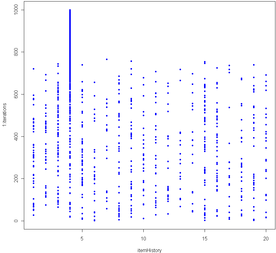
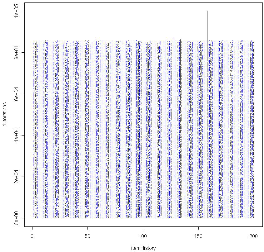
The graph above shows the results of 1000 iterations with 20 balls (each victory increases the weight of the winner by 5%). The more balls you have, the longer it takes before a clear winner appears. Here’s the graph for 200 balls (0.5% weight boost for each victory).

As you can see, in this simulation it took about 85,000 iterations before a clear winner appeared.

I contend that as the number of iterations grows, the probability of seeing a Chosen One approaches unity, no matter how many balls you use. In other words, for any number of balls, a single one of them will eventually see its relative weight, compared to the others, diverge. Can you prove this is true?

BTW this is a good Monte Carlo simulation of the Matthew Effect (no relation).

Here is the code in R to replicate:

numbItems = 200
items = 1:numbItems
itemWeights = rep(1/numbItems,numbItems) # Start out uniform
iterations = 100000
itemHistory = rep(0,iterations)

for(i in 1:iterations) {
	chosen = sample(items, 1, prob=itemWeights)
	itemWeights[chosen] = itemWeights[chosen] + (itemWeights[chosen] * (1/numbItems))
	itemWeights = itemWeights / sum(itemWeights) # re-Normalze
	itemHistory[i] = chosen
}

plot(itemHistory, 1:iterations, pch=".", col="blue")

After many trials using a fixed large number of balls and iterations, I found that the moment of divergence was amazingly consistent. Do you get the same results?


12
Jun 10

A different way to view probability densities

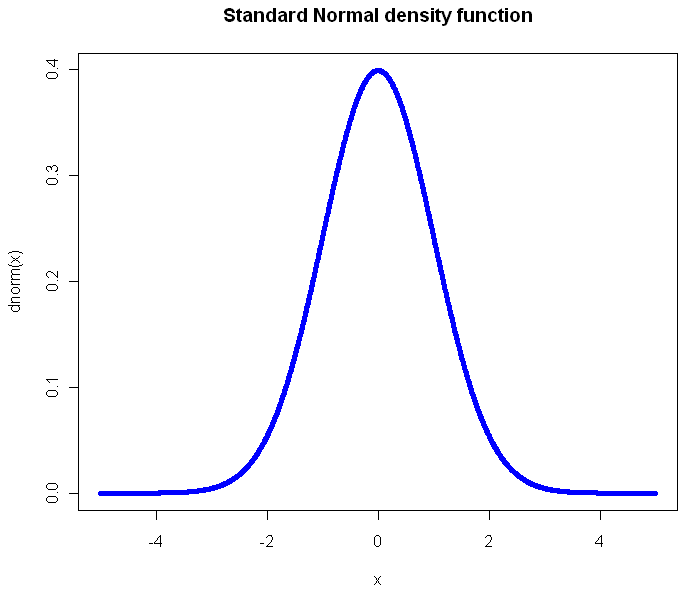
The standard, textbook way to represent a density function looks like this:

Perhaps you have seen this before? (Plot created in R, all source code from this post is included at the end). Not only will you find this plot in statistics books, you’ll also see it in medical texts, sociology, and even economics books. It gives you a clear view of how likely an observation is to fall in a particular range of [latex]x[/latex]. So what’s the problem?

The problem is that what usually concerns us isn’t probability in isolation. What matters is the impact that observations have on some other metric of importance, like the total or average. The key thing we want to know about a distribution is: What range of observations will contribute the most to our expected value, and in what way? We want a measure of influence.

Here’s the plot of the Cauchy density:

From this view, it doesn’t look all that different from the Normal. Sure it’s a little more narrow, with “fatter tails”, but no radical difference, right? Of course, the Cauchy is radically different from the normal distribution. Those slightly fatter tails give very little visual indication that the Cauchy is so extreme-valued that it has no expected value. Integrating to find the exception gives you infinity in both directions. If your distribution is like this, you’ve got problems and your plot should tell you that right away.

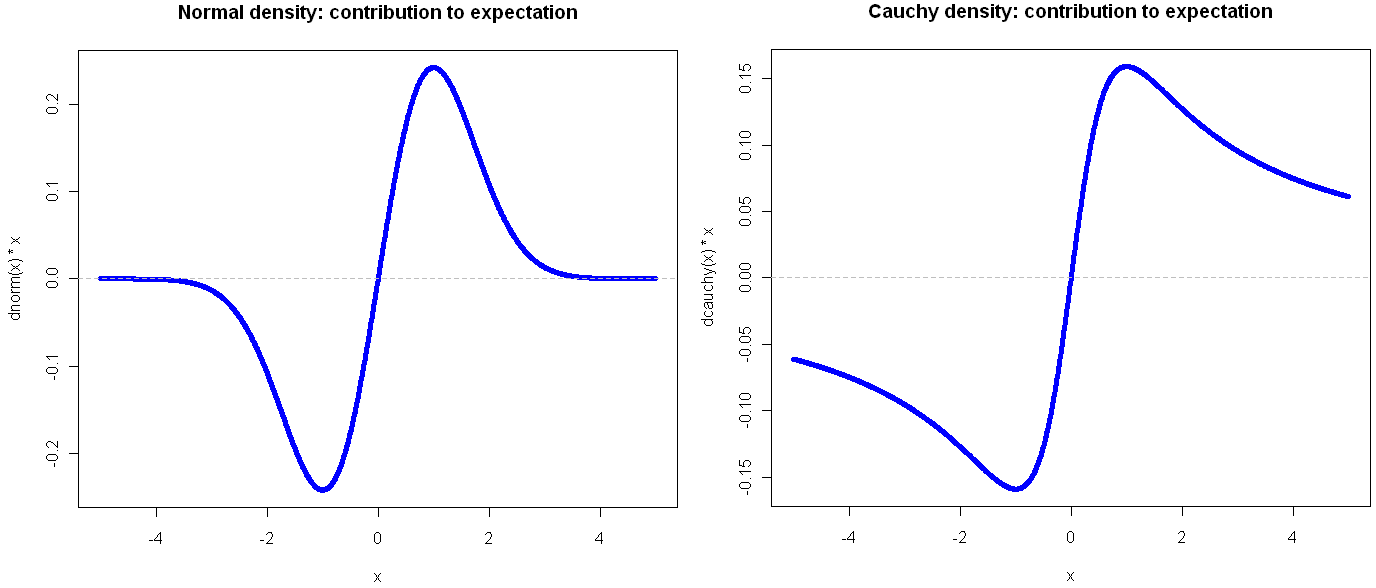
Here’s another way to visualize these two probability distributions:

Go ahead and click on the image above to see the full view. I’ll wait for you…

See? By plotting the density multiplied by the observation value on the y-axis, you get a very clear view of how the different ranges of the function effect the expectation. Looking at these, it should be obvious that the Cauchy is an entirely different beast. In the normal distribution, extreme values are so rare as to be irrelevant. This is why researchers like to find ways to treat their sample as normally distributed: a small sample gives enough information to tell the whole story. But if your life (or livelihood) depends on a sum or total amount, you’re probably best off plotting your (empirical) density in the way shown above.

Another bit of insight from this view is that the greatest contribution to the expectation comes at 1 and -1, which in the case of the Normal isn’t the mean, but rather the second central moment (plus or minus). That’s not a coincidence, but it’s also not always the case, as we shall see. But first, what do things look like when a distribution gets completely out of hand?

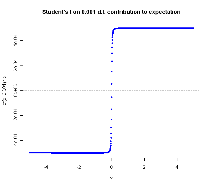
The Student’s t distribution, on 1 Degree of Freedom , is identical to the Cauchy. But why stop at a single DF? You can go all the way down to the smallest (positive) fraction.

The closer you get to zero, the flatter the curve gets. Can we ever flatten it out completely? Not for a continuous distribution with support over an infinite range. Why not? Because in order for the slope of [latex]value * density[/latex] to continue to flatline it indefinitely, the density function would have to be some multiple of [latex]\frac{1}{x}[/latex], and of course the area under this function diverges as we go to infinity, and densities are supposed to integrate to 1, not infinity, right?

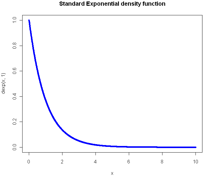
What would the plot look like for a continuous function that extends to infinity in just one direction? Here’s the regular Exponential(1) density function plot:

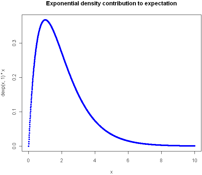
Now look at the plot showing contribution to expectation:

Were you guessing it would peak at 1?  Again, the expectation plot provides insight into which ranges of the distribution will have the greatest impact on our aggregate values.

Before I go look at an a discrete distribution, try to picture what the expectation curve would look like for the standard [latex]Uniform(0,1)[/latex] distribution. Did you picture a diagonal line?

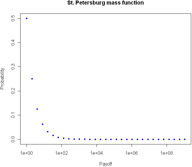
Can we flatten things out completely with an infinitely-supported discrete distribution? Perhaps you’ve heard of the St. Petersburg Paradox. It’s a gambling game that works like this: you flip a coin until tails comes up. If you see one head before a tails, you get $1. For 2 heads you get $2, for 3 heads $4, and so on. The payoff doubles each time, and the chances of reaching the next payoff are halved. The paradox is that even though the vast majority of your winnings will be quite modest, your expectation is infinite.  The regular view of the probability mass function for provides almost no insight:

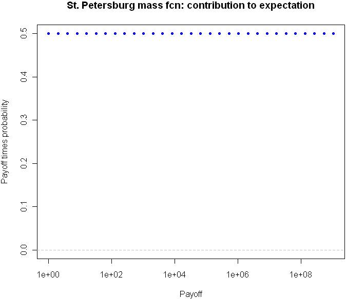
But take a look at the expectation plot:

Flat as a Nebraska wheat field. You can tell right away that something unusual is happening here.

I could go on with more examples, but hopefully you are beginning to see the value in this type of plot. Here is the code, feel free to experiment with other distributions as well.

# Useful way to make dots look like a line
x = seq(-5,5,length=1500)

# You've seen this before. Our good friend the Normal
plot(x,dnorm(x),pch=20,col="blue", main="Standard Normal density function")

# Cauchy looks a little different, but it's not obvious how different it is 
plot(x,dcauchy(x),pch=20,col="blue", main="Cauchy density function")

# New way of plotting the same
plot(x,dnorm(x)*x,pch=20,col="blue", main="Normal density: contribution to expectation")
abline(h=0,lty="dashed",col="gray")

plot(x,dcauchy(x)*x,pch=20,col="blue", main="Cauchy density: contribution to expectation")
abline(h=0,lty="dashed",col="gray")

# Extreme student-t action:
plot(x,dt(x,0.001)*x,pch=20,col="blue", main="Student's t on 0.001 d.f. contribution to expectation")
abline(h=0,lty="dashed",col="gray")


# The Exponential
x = seq(0,10,length=1500)
plot(x,dexp(x,1),pch=20,col="blue", main="Standard Exponential density function")

# The expectation view:
plot(x,dexp(x,1)*x,pch=20,col="blue", main="Exponential mass contribution to expectation")

# What do we see with the St. Petersburg Paradox
x = 2^(0:30)
dStPete <- function(x) {
	return (1/(2*x))
}

# Note the log
plot(x,dStPete(x),pch=20,col="blue", main="St. Petersburg mass function", log="x", xlab="Payoff", ylab="Probability",ylim=c(0,.5))

# Now we see the light
plot(x,dStPete(x)*x,pch=20,col="blue", main="St. Petersburg mass fcn: contribution to expectation", xlab="Payoff", log="x", ylab="Payoff times probability",ylim=c(0,.5))
abline(h=0,lty="dashed",col="gray")

30
Apr 10

How many girls, how many boys?

I found this interesting question over here at mathoverflow.net. Here’s the question:

If you have a country where every family will continue to have children until they get a boy, then they will stop. What is the proportion of boys to girls in the country.

First off, there are some assumptions you need to make that aren’t stated in the problem. The most important one is that boys are just as likely as girls to be born. This is empirically false, but there’s nothing wrong with assuming it for the problem, so long as the assumption is acknowledged.

My first thought about solving the problem was to think about Martingales and stopping times, but that’s more complication than you need. If you look at it from the point of view of expectation things are simpler.The probability of having a boy first is 1/2, at which point the family stops and you have a ratio of 1 boy per 1 births. The probability of having one girl, then one boy is 1/4, at which point you have a ratio of 1 boy per 2 births. Multiplying the probabilities by the ratios and summing from 1 birth to infinity, you get an expectation of approximately 69.31% boys.

Problem is, this is the expectation for a single family. Because families who have more children (and thus more girls) contribute disproportionately to the pool of children, one family is a biased estimator for the proportion in the entire population. Douglas Zare at the above-linked mathoverflow question does a good job of working out the details for a country with an arbitrary number of families. Here is what he comes up with for the percentage of girls:

Where k is the number of families in the country, and  is the digamma function.

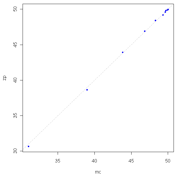
To be true to the new motto of this site, I decided to test this out in R using a Monte Carlo method. Here is my code:

And here is the resulting graph:

Looks like a good match.

Maybe you noticed that at the beginning I mentioned assumptions, as in more than one. We are also assuming that that all of the boys and girls, no matter how old, are still considered boys and girls. All of the parents were already in the country at the beginning of the problem, and then they all started having children until they had a boy and stopped. None of these children have had any children. The process is complete, and the new generation is the last. Obviously even if parents in a country did follow the rule of "babies until boy then stop", the results wouldn't match the theoretical because at any given moment there are many families in the process of still having kids. This is where, if I were so inclined or needed a more accurate model, I would dive back into the Martingale issue and things would get messy.