Probability and statistics blog

I woke up from my afternoon nap feeling a bit off-kilter, so I decided to go for another random walk. In particular, I wanted a journey that avoided the center, but didn’t just run for an exit either. After playing around for a while I came up with this:

# Take a wacky walk, return the final "track" steps
wackyWalk <- function(iters, track=iters) {
	locations = c()
	mean2use = 0
	sd2use = 1

	for (i in 1:iters) {
		mean2use = rnorm(1,mean2use,sd2use) 

		# The farther from the center, the smaller the variance
		sd2use = abs(1/mean2use)
		if(track > (iters - i) ) {
	 		locations = c(locations, mean2use)
	 	}
	}
	return(locations)
}

# How many steps to take
iters = 300
track = 300
locations = wackyWalk(iters,track)

# Start us off with a plot
plot(0,0,xlim=c(min(locations),max(locations)),ylim=c(0,iters),pch=20,col="white")

for (i in 1:track) {
	points(locations[i],i,pch=20,col="blue")

	# To create a pseudo animation, take a break between plotting points
	Sys.sleep(.10)
}

Basically, during each iteration the program samples from a normal distribution centered at the same location as the previous iteration, with standard deviation equal to the inverse of the previous location. So if the sequence is at 5, the next number will be sampled from the [latex]Normal(5, (\frac{1}5)^2)[/latex] distribution.

Run it a few times and you’ll see how the blue dot bounces around for a bit near 0, then shoots off to one side or the other, where it will most likely hang out for the rest of its life. There are a number of interesting questions about this sequence which, sadly, will remain unanswered. Among these are: For a given number of iterations, how many times is this sequence expected to cross zero? What is the maximum (or minimum) value the sequence is expected to obtain over a fixed number of iterations? Will the sequence ever diverge to some flavor of infinity?

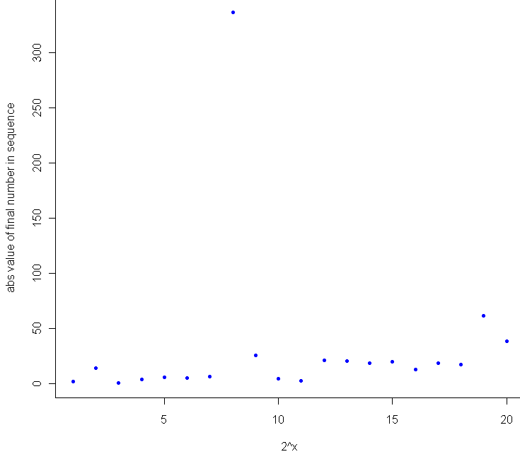
My hunch for this last question is to say no, since the normal distribution is thin-tailed, and the standard deviation is set to converge to 0 (slowly) as the value of the sequence gets larger and larger. At the same time, I suspect that the higher the number of iterations, the larger (in absolute terms) the final number in the sequence. This makes general sense, as the farther you get from 0, the harder it is to return to 0. During testing, I saw a lot of plots that wiggled back and forth, getting closer to the edges of the plot with each wiggle. Since I’m never content to just have a thought without actually testing it out, I plotted the final value in the sequence after [latex]2^x[/latex] iterations, where x went from 1 to 20. Here’s the result:

Sure enough, as a general trend, the more iterations you run, the farther you are from zero. It would have been interesting to see how the 8th trial ended up north of 300, but I only tracked the final result for these. I suspect that it made up most of the ground in a single leap while sampling from a Normal with extremely high variance (ie when the previous number was very close to 0).

Here’s the extra bit of code for comparing final location to number of iterations:

# How does the number of steps compare with distance from center
meta = c()
for (j in 1:20) {
	iters = 2^j
	track = 1
	meta = c(meta, wackyWalk(iters,track))
}

plot(1:20, abs(meta), pch=20, col="blue",xlab="2^x",ylab="abs value of final number in sequence")

These results, I should note, provide very little evidence that the sequence, if extended out to infinite length, will have to converge or diverge. Weird things happen when you start to consider random walks of infinite length, and the one sure limitation of Monte Carlo testing is that no matter how long let a computer simulation run, your PC will crash well before it performs an infinite number of calculations, and most likely before you finish your coffee.