I was reading over at math-blog.com about a concept called numeri ritardatari. This sounds a lot like “retarded numbers” in Italian, but apparently “retarded” here is used in the sense of “late” or “behind” and not in the short bus sense. I barely scanned the page, but I think I got the gist of it: You can make money by betting on numbers which are late, ie numbers that haven’t shown up in a while. After all, if the numbers in a lottery or casino are really random, that means it’s highly unlikely that any one number would go a long time without appearing. The “later” the number, the more likely it is to appear. Makes sense, right?
Before plunking down my hard(ly) earned cash at a casino, I decided to test out the theory first with the prototypical random number: Pi. Legend has it that casinos once used digits from Pi to generate their winning numbers. Legend also has it that the digits of Pi are so random that they each appear with almost exactly 1 in 10 frequency. So, given this prior knowledge that people believe Pi to be random, with uniform distribution of digits and no discernible pattern, I can conclude that no one digit should go too long without appearing.
I pulled down the first 10 million digits from here (warning, if you really want this data, right click the link and “save as”). Then I coded up a program in the computer language R to scan through the digits of Pi, one by one, making a series of “fair” bets (1:9 odds) that the next number to appear in the sequence would be the one that had gone longest without appearing. My code is shown below. I had to truncate the data to 1 million digits, and even then this code will take your Cray a good while to process, most likely because I have yet to master the use of R’s faster “apply” functions with complicated loops.
myPi = readLines("pi-10million.txt")[1]

# I think this is how I managed to get Pi into a vector, it wasn't easy.
piVector = unlist(strsplit(myPi,""))
piVector = unlist(lapply(piVector,as.numeric))

# In honor of Goofy Programming Day, I will
# track how long since the last time each digit appeared
# by how many repetitions of that digit are in a vector
ages = c()

# Start us off with nothing in the bank
potHistory = c()

# R just loves long loops like this. Hope you have a fast computer
for(i in 1:1000000) {
	# How did our bet do last round?
	# Skip the first 100 just to build up some data
	if(i > 100) {
		if(betOn == piVector[i]) {
			potHistory = c(potHistory, 9)
		} else {
			potHistory = c(potHistory, -1)
		}
	}

	# Increase all ages by 1 by adding to vector, then set the one we found to 0
	ages = c(ages, 0:9)
	ages = ages[!ages == piVector[i]]

	# Count occurences of each digit, find the top digits by occurence to bet on
	# And you thought Perl was beautiful?
	betOn = as.numeric(names(sort(-table(ages)))[1])
}

# Plot the cumulative sum at 1000 point intervals.
plot.ts(cumsum(potHistory)[seq(0,1000000,500)],pch=20,col="blue",xlab="step/500",ylab="cumulative earnings")
So what was the result? How good was my strategy? After an initial 100 digits to build up data about which digits were latest, I placed a total of 999,900 bets at $1 each. Final earnings: $180. That’s so close to breaking even that it’s almost inconceivable. I had 100,008 wins and 899,892 losses. My winning percentage was 10.0018% percent.
On the face of it, this result seemed almost a little too good, dare I say even suspiciously good, if you know what I mean. How rare is it to get this close (or closer) to the exact perfect proportions after so many trials? Assuming that the number of wins followed a binomial distribution with [latex]p=0.1[/latex], my total wins should follow a Normal distribution with mean 99,990 and variance [latex]n*p*(1-p) = 89,991[/latex] (for an “n” of almost a million and non-minuscule “p”, the Normal approximation to the Binomial should be essentially perfect). Taking the square root of the result, and we get almost exactly 300 as our standard deviation. That’s much larger than the 18 extra wins I had. In fact, the chances that you will land within [latex]18/300 = 0.06[/latex] standard deviations on either side of the Normal’s mean are less than 5%. Before getting too worked up over this result, I decided to take a look at the graph. Using the code:
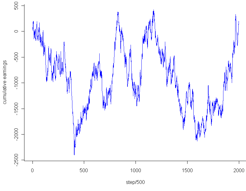
plot.ts(cumsum(potHistory)[seq(0,1000000,500)],pch=20,col="blue",xlab="step/500",ylab="cumulative earnings")
I got this:
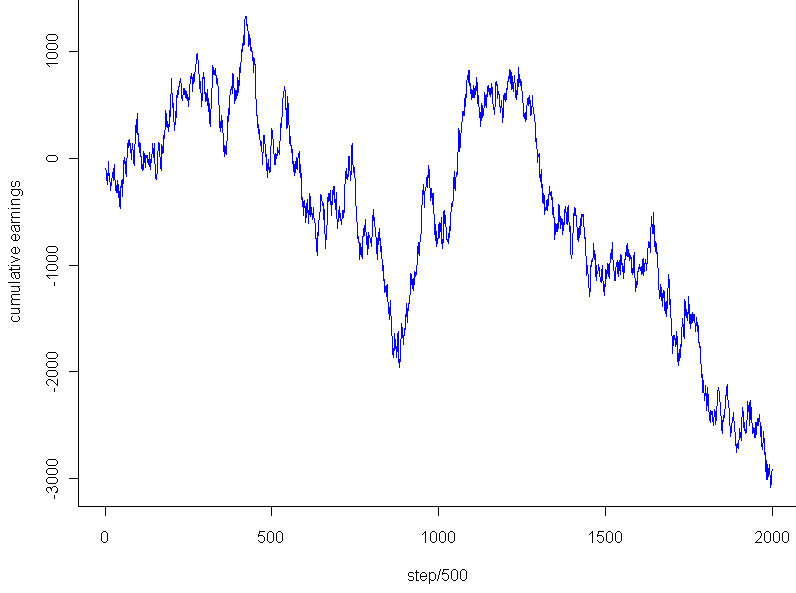
The graph looks pretty much like any random walk, doesn’t it? So the fact that I ended up breaking almost exactly even had to do with the stopping point, not any “unusual” regularity. Just to see if I might salvage any mystery, I tested the very lowest point, -$2,453, which occurred after 202,133 trails. Even that falls within 2 standard deviations of the expected mean for that number of trials, and of course cherry picking the most extreme point to stop at isn’t a fair way to go about this. Any last hope that the graph might be unusual? I plotted a couple random walks using numbers generated in R. Most of them looked like this:
This looks to have the same level of “jaggedness” as the results of my bet on Pi. Unfortunately, I am forced to conclude that the promising strategy of “late number” gambling turned out to be fairly retarded after all, at least so far as it applies to the digits of Pi.


