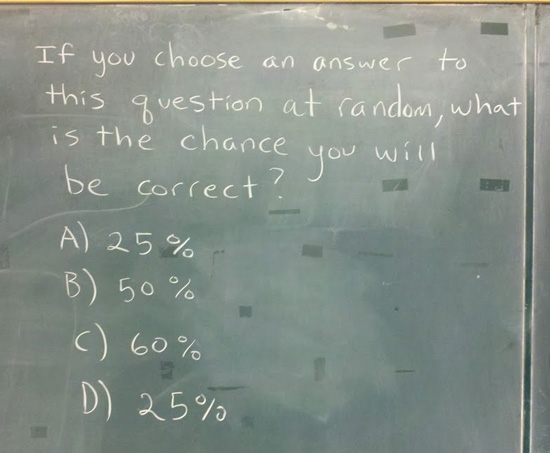
Image found out there on The Internets. If it doesn’t hurt your brain, you’re not thinking about it hard enough.
feature
13
Oct 12
If you choose an answer to this question at random, what is the chance you will be correct?
13
Oct 12
The unicorn problem
Let’s say your goal is to observe all known species in a particular biological category. Once a week you go out and collect specimens to identify, or maybe you just bring your binoculars to do some spotting. How long will it take you to cross off every species on your list?
I’ve been wondering this lately since I’ve begun to hang out on the Mushrooms of Québec flickr group. So far they have over 2200 species included in the photos. At least one of the contributors has written a book on the subject, which got me wondering how long it might take him to gather his own photos and field observations on every single known species.
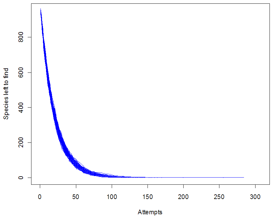
My crude model (see R code at the end of this post) assumes that every time Yves goes out, he has a fixed chance of encountering every given species. In other words, if there were 1000 species to find, and he averages 50 species per hunt, then every species is assigned a 1/20 chance of being found per trip. Thus the total found on any trip would have a Poisson distribution with parameter 50.
This model is unrealistic for lots of reasons (can you spot all the bad assumptions?), but it does show one of the daunting problems with this task: the closer you get to the end, the harder it becomes to find the last few species. In particular, you can be stuck at 1 for a depressingly long time. Run the simulation with different options and look at the graphs you get. I’m calling this “The unicorn problem,” after Nic Cage’s impossible-to-rob car in the movie Gone in 60 Seconds.
Do you have a real-life unicorn of one sort or another?
species = 1000
findP = 1/20
trials = 100
triesToFindAll = rep(0, trials)


for(i in 1:trials) {
	triesNeeded = 0

	leftToFind = rep(1, species)
	leftNow = species
	numberLeft = c()

	while (leftNow > 0) {

		found = sample( c(0,1), 1000, replace=TRUE, prob = c((1-findP),findP))

		leftToFind = leftToFind - found

		leftNow = length(leftToFind[leftToFind > 0])

		numberLeft = c(numberLeft, leftNow)

		triesNeeded = triesNeeded + 1

	}

	if(i == 1) {
		plot.ts(numberLeft, xlim=c(0, 2*triesNeeded), col="blue", ylab="Species left to find", xlab="Attempts")
	} else {
		lines(numberLeft, col="blue")
	}

	triesToFindAll[i] = triesNeeded
}
19
Jun 12
Manifesto update
A small one in terms of words, but lots of thought has gone into this addition:
Correlation proves compatibility.
Negative correlation implies incompatibility.
As Ned Ryerson would ask, “Am I right or am I right?”
3
May 12
Early May Link roundup
Naomi Robbins looks at using pie charts to represent women and men in publishing. Her piece is here. The charts in question are here. Warning: Don’t click if you hate pie charts, you just might have a meltdown or wonder why all the info couldn’t be put into a single bar chart.
Discussion at Cross Validated about How best to communicate uncertainty with way too few responses. My feeling is that as news filters from scientific realms to pop culture outlets, it becomes more and more “certain” in terms of how it’s presented. Can that be fixed?
Master of data visulization Hans Rosling made Time magazines list of 100 most influential people in the world.
2
May 12
May Manifesto addendum
Just added another statement to my manifesto. Here is the full text:
Interpret or predict. Pick one. There is an inescapable tradeoff between models which are easy to interpret and those which make the best predictions. The larger the data set, the higher the dimensions, the more interpretability needs to be sacrificed to optimize prediction quality. This puts modern science at a crossroads, having now exploited all the low hanging fruit of simple models of the natural world. In order to move forward, we will have to put ever more confidence in complex, uninterpretable “black box” algorithms, based solely on their power to reliably predict new observations.
Since you can’t comment to WordPress pages, you can post any comments about my latest addition here. First, though, here is an example that might help explain the difference between interpreting and predicting. Suppose you wanted to say something about smoking and its effect on health. If your focus is on interpretability, you might create a simple model (perhaps using a hazards ratio) that leads you to make the following statement: “Smoking increases your risk of developing lounge cancer by 100%”.
There may be some broad truth to your statement, but to more effectively predicts whether a particular individual will develop cancer, you’ll need to include dozens of additional factors in your model. A simple proportional hazards model might be outperformed by an exotic form of regression, which might be outperformed by a neural network, which would probably be outperformed by an ensemble of various methods. At which point, you can no longer claim that smoking makes people twice as likely to get cancer. Instead, you could say that if Mrs. Jones —a real estate agent and mother of two, in her early 30s, with no family history of cancer — begins smoking two packs a day of filtered cigarettes, your model predicts that she will be 70% more likely to be diagnosed with lounge cancer in the next 10 years.
The shift taking place right now in how we do science is huge, so big that we’ve barely noticed. Instead of seeing the world as a set of discrete, causal linkages, this new approach sees rich webs of interconnections, correlations and feedback loops. In order to gain real traction in simulating (and making predictions about) complex systems in biology, economics and ecology, we’ll need to give up on the ideal of understanding them.
23
Feb 12
A classification scheme for types of randomness
We often speak implicitly of different types of randomness but neglect to name or categorize them. Consider this post to be a kind of white paper or rough draft on the division of randomness into five categories. If you start using these distinctions explicitly, even if only in your own head, I think you will find them highly useful, as I have.
Type 0: Fixed numbers or known outcomes
Type 0 randomness is the special case of randomness where the data are already known. Any known outcome, regardless of the process that generated it, is Type 0 randomness. Once known, it has become a constant. In terms of information conveyed, all Type 0 randomness has zero informational entropy (a measure of uncertainty), and all messages with zero entropy are examples of Type 0 randomness.
Type 1: Pseudo random.
Most computers generate random numbers by a deterministic process. An initial “seed” is picked using some environmental factor, like the microsecond timing of the CPU, and from there onward every number that follows is fully determined by the algorithm. These algorithms can be very good, in terms of producing sequences of numbers that have desirable qualities. Yet, if you know that the sequence comes from some variation of, say, the Mersenne Twister, then a single number or short sub-sequence might be enough to predict all the subsequent numbers. Even if you can’t guess at the underlying mechanism, algorithms like the Mersenne Twister eventually loop: once you’ve seen the whole sequence, all future numbers will be known exactly, and you will have Type 0 randomness.
Computer software isn’t the only source of Type 1 randomness. Card shuffling machines, if sufficiently precise in their operation, map each unique ordering of playing cards to a single final ordering. Learn how the machine works, and you will know how each initial ordering is transformed.
The key to Type 1 randomness is that it is fully reducible to Type 0, in principle. The data source is known to be determinate, but the code is yet to be cracked. With enough time, attention, or technical sophistication, the sequence can be fully mapped.
Type 2: Non-fully reducible
Most real world randomness, and in general the most interesting sources of randomness, are of Type 2. Data streams of Type 2 randomness are conditionally random in the sense that we are able to reduce the uncertainty related to them, but only up to a certain point. Our model predicts the value of some response variable based on the other data, and this prediction can be quite good. But with Type 2 randomness there will always be some uncertainty left over, conditional on us making the best prediction we can.
A typical example of Type 2 randomness would be predicting whether certain individuals will develop heart disease within the next 10 years. Without knowing any specifics about the individuals, it’s very hard to make accurate predictions. Once we know some basic data, such as age, sex, and weight, we can make a better prediction. Even more fine-grained detail — history of smoking, diet, exercise patterns — allow us to make even better predictions. Each study or experiment we do, if of sufficient quality, improves the predictions we are able to make. Yet the randomness is non-fully reducible in the sense that, no matter how good our prior information or model, we will never be able to predict with 100% certainty whether a person will develop heart disease.
Regression curves are attempts to understand Type 2 randomness by separating signal (the model, or conditionally determinant, part) and noise. Often this noise part is modeled with some maximum entropy distribution, like the Gaussian. This is our way of recognizing that beyond some limit, we can no longer reduce the randomness. There will always be some Type 3 randomness left over.
Type 3: Martingale random
One way to think about Type 3 randomness is to imagine a fair bet. If the true probability of an event happening is 1/2, then 1 to 1 odds make it martingale random. There’s nothing you can do to improve your expected return to above zero; nor is there anything you can do to decrease your exception to below zero. In a series of independent fair bets, strategy is irrelevant to expectation. Importantly, this doesn’t prevent you from adjusting the probability distribution for payoffs, if you are able to vary wager amounts and stopping times. For example, you could try the martingale betting strategy, which offers a high probability of making small gains in exchange for a small chance of catastrophic loss.
Martingale randomness implies that there is no disconnect between the “advertised” distribution and the true (or revealed) distribution. The theoretical “fair coin” you meet in textbooks is martingale random. Of course you have to be very careful in how you interpret the results of a real coin toss in terms of informational content. Maybe it isn’t martingale random after all!
Type 3 randomness is not limited to situations in which you have two equally probable outcomes. Anytime you are unable to reduce randomness beyond a particular limit of predictability, what’s left over is martingale randomness. In fact, through a process of “whitening,” signals that generate non-uniform randomness can be converted into uniform randomness. The opposite can be accomplished as well (though I’ve never heard it called “blackening”).
Type 4: Real randomness.
This is the real thing: baked-in, irreducible randomness. For a data source to be Type 4 random, it must be martingale random and it must come from a sequence that is not only unknown, but a priori unknowable. If Type 4 randomness exists, then God plays dice; randomness is “baked in” to the universe.
I suspect that if Type 4 randomness really does exist, then it will be impossible to prove.
General thoughts on types and some examples
The most important thing to note about these categorizations is that the type of randomness depends on your perspective. The cards you hold in your hand are Type 0 randomness to you, but to the person sitting across the poker table from you, they are Type 2 randomness. Your opponent can use any number of tools to try and do better than pure chance at guessing your hand (how much you bet, the look in your eyes, and of course the cards they hold). The type of randomness you perceive is a function of what you know.
All degenerate random variables (i.e. the indicator function for the entire sample space, which is always 1) are Type 0 randomness.
Most of the games we play have some element of Type 2 randomness. Kids will play games with Type 1 randomness, like War, which is deterministic for any given card shuffling, and could in theory be mapped out. Type 1 randomness can still be surprising to you, but if there is any skill involved it would have to be Type 2 randomness: entropy reducible in theory.
The concept of Type 3 randomness is connected with two important statistical concepts: sufficiency and coherence. Once you know the sufficient statistics from a data source (and, vitally, assuming your model about the data is correct), threre’s nothing more you can do to improve your confidence intervals or ability to make predictions. For example, if you know that your data source has a Poisson distribution and the points are uncorrelated, then once you know the mean, there’s no other piece of information that can improve your ability to predict new values from the distribution. Broadly speaking, martingale randomness satisfies the de Finetti conditions of coherence, in that odds assignments must match up with known probabilities, and internal consistency needs to be maintained.
If your dice are loaded, then you’ve got a generator of Type 2 randomness. Over time, you can make better and better predictions about how often the different numbers will come up. But you still won’t be able to predict, with certainty, the results of any given roll. If somehow you knew the exact probabilities for each face, then you could use these dice as a generator of Type 3 randomness.
In a sense, the very first number generated by your computer’s random number algorithm is martingale random. There’s no way, unless you know how the seed is generated from the CPU’s timing and can “see” the microseconds tick by, to predict the range in which that number will fall with greater accuracy than would be expected by chance alone. On the other hand, it could be argued that the decimal part of the CPU’s clock isn’t really uniformly distributed. There will be some slight bias towards lower numbers, which is natural for any distribution of numbers that “grows” in size, even if it cycles (see Benford’s Law, and note that it applies not just to the first digit of a number, but to secondary digits as well). With enough careful investigation, you might be able to convert that first seeded random number into a case of Type 2 randomness.
Type 3 randomness is the holy grail of randomization. Casinos want dice which are perfectly symmetric in weighting, and resistant to wear and tear that might cause bias. Assignments to treatment in a clinical trial should strive for martingale randomness. Failure to achieve martingale randomness, when it is required, can have highly negative consequences.
“Beating the house” at a casino involves turning Type 3 randomness into Type 2 randomness, with enough usable signal left to overcome the casino’s inherent advantage. Strategies like analyzing roulette spins to find bias, and most famously counting cards, have been successfully used. One group of geeks was able to turn the randomness of a Vegas lottery machine which followed a Type 1 sequence into Type 0. They made the tactical mistake of hitting two huge jackpots in a row, tipping off the casino that they had successfully cracked the code. From the casino’s perspective, you have an inverse classification problem: given how well players are doing, what can you infer about the type of randomness they are detecting? Those jackpot-winning geeks could have taken a lesson from code breakers in WWII, who thought carefully about how to use the information contained in the cracked messages without showing the Germans that their code had been broken and that the allies understood their messages as more than the white noise of Type 3 randomness.
Because what separates the Types is our knowledge, randomness can come from a generation process that is completely deterministic and known to others (Type 0). As far as I’ve been able to tell, the digits of pi (beyond the ones you have memorized) are martingale random. If I give you a sequence of digits, and tell you they come from somewhere after the trillionth digit of pi, and let you use any tools you want short of a computer, there’s nothing you could do in a single lifetime to predict additional digits with an accuracy greater than 1/10th. Note that while the tail digits of pi appear to be a source of martingale randomness, not all irrational (or even transcendental) numbers have unpredictable digits. As counterexamples, see Louisville’s or Chapperhorn’s numbers. Any data source of Type 2 or greater must be incompressible, in the sense that if the sequence has infinite length, no finite-length description of it can exist. If there were a finite-length algorithm that could re-create (or predict) the sequence, then it’s at most Type 1 randomness (until we figure out this algorithm, if need be by iterating over all possible algorithms, starting with the shortest, until we get there).
I’ve tried to make these categorizations as clear as possible, but there are still edge cases which are hard to place. As is always the case, the closer you look, the fuzzier things get. However, I think you will still find this categorization of randomness to be quite useful, especially as a tool to discuss edge cases. Consider for a moment Chaitin’s Omega, which is the probability (weighted by string length) that a given computer program, run in a fixed computing environment, halts. The first few digits of Omega, determined by very short programs which instantly halt or loop, are easy to figure out. But we know from Turing that the halting problem is, in general, undecidable. So at some point, the digits of Omega become unknown and unknowable. Nor can we know when they become unknowable! The digits of Omega make the transition from Type 0 randomness (known) to Type 1 randomness (we just need to run the programs and see if they halt or loop), to Type 2 randomness (we may be able to set upper and lower bounds for the next few digits, or make a likelihood prediction based on reasoning and past experience), to Type 3 randomness (only God could predict the 10,000th digit with better than chance accuracy) and perhaps, almost frighteningly, to Type 4 randomness (God’s in a back alley, shaking up the dice right now).
15
Jan 12
R A Fisher illustration

Ronald Aylmer Fisher, statistics badass. Illustration by Rachelle Scarfó for a project I was working on.
6
Jan 12
Explaining large numbers
It can be very hard to convey the meaning and importance of large numbers. As Joseph Stalin infamously said (or perhaps didn’t): “The death of one man is a tragedy. The death of a million is a statistic.” The point being that we can conceive of one person dying, perhaps our mother or a friend. We can understand it and feel it. However horrific the deaths of a million, the size of the number itself turns it into an abstraction.
The video above explores a concept that is abstract to begin with (the national debt) and made even more incomprehensible by having an impossibly large number attached to it (15 trillion). So, how do you make an abstract idea and a massive number meaningful? By personalizing it.
I like the video’s approach, but like other attempts to dividing up a huge number into individual shares, a certain amount of dishonesty is involved. Nation debt, of course, isn’t the same as family debt. For one thing, your family can’t just print more money (though in some ways the availability of a printing press means the national debt is even more scary). Also, there is a big difference between one family living beyond its means and, by extension, every single family in the country living beyond its means.
4
Jan 12
Iowa: Was the fix in? (a statistical analysis of the results)
Summary/TL;DR
Either the first precincts to report were widely unrepresentative of Iowa as a whole, or something screwy happened.
Background
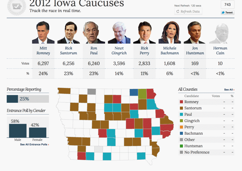
Yesterday was the first primary for the 2012 U.S. presidential elections. When I logged off the internet last night, the results in Iowa showed a dead heat between Ron Paul, Mitt Romney, and Rick Santorum. When I woke up this morning and checked the results from my phone, they were very different. So before connecting to the internet, I took a screen shot of what I saw before going to bed. Here it is:
Then I connected to the internet and refreshed that page:
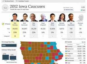
It seemed strange to me that the results should change so dramatically after 25% of the votes had already been recorded. As a statistician, my next question was: how unusual is this? That’s a question that can be tested. In particular, I can test how often you might have a split of voters like the one shown in the first screen shot, if the final split is like the one shown in the other screen shot, given that the first precincts to report were similar to later ones in voter composition.
That’s a lot to digest all at once, so I’m going to repeat and clarify exactly what I’m assuming, and what I’m going to test.
The assumptions
First, I assume the following:
1. That CNN was showing the correct partial results as they became available. Similarly, I am assuming that the amount shown with 99% of votes reported (second screen shot) is the true final tally, give or take some insignificant amount.
2. That the precincts to report their vote totals first were a random sampling of the precincts overall. Given how spread out these appear to be in the first screen shot, this seems like a good assumption. But that might not be the case. See the end of this post for more about that possibility.
3. No fraud, manipulation, or other shenanigans occurred in terms of counting up the votes and reporting them.
The test
Given these three assumptions, I’m going to come up with a numeric value for the following:
1. What is the probability that the split, at 25% of the vote tallied, would show Ron Paul, Mitt Romney, and Rick Santorum all above 6,200 votes.
It’s possible to come up with a theoretical value for this probability using a formal statistical test. If you decide to work this out, make sure to take into account the fact that your initial sample size (25%) is large compared to the total population. You’ll also need to factor in all of the candidates. Could get messy.
For my analysis, I used the tool I trust: Monte Carlo simulation. I created a simulated population of 121,972 votes, with 26,219 who favor Ron Paul, 30,015 who favor Mitt Romney, and so on. Then I sampled 27,009 from them (the total votes tallied as of the first screen shot). Then I looked at the simulated split as of that moment, and saw if the three top candidates at the end are all above 6,200 votes. What about just Ron Paul?
I’ve coded my simulation using the programming language R, you can see my code at the end of this post.
The results
Out of 100,000 simulations, this result came up not even once! In all those trials, Ron Paul never broke 6,067 votes at the time of the split.
I ran this test a couple times, and each time the result was the same.
Conclusion
If my three assumptions are correct, the probability of observing partial results like we saw is extremely small. It’s much more likely that one of the assumptions is wrong. It could be that the early reports were wrong, though that seems unlikely. The other websites showed the same information or very similar, so it seems doubtful that an error occurred in passing along the information.
Was there something odd about the precincts that reported early? This is not something you could tell just by looking at split vs final data. The data clearly show that the later precincts disfavored Ron Paul, but that’s just what we want to know: did they really disfavor him, or was the data manipulated in some way. The question is, were any of the results faked, tweaked, massaged, Diebold-ed?
To answer that question, we’d need to know if these later precincts to report were expected, beforehand, to disfavor Ron Paul relative to the others. It would also help to look at entrance polling from all of the precincts, and compare the ones that were part of the early reporting versus those that were part of the later reports. At this point, I have to ask for help from you, citizen of the internet. Is this something we can figure out?
UPDATE
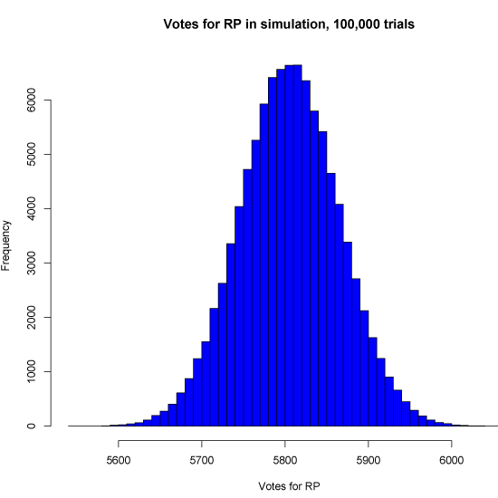
In case folks are interested, here’s a histogram of the 100,000 simulations. This shows the distribution of votes for Ron Paul as of the split, given the assumptions. As you can see it’s a nice bell curve, which it should be. Also note how far out on the curve 6,240 would be.
The code
Oh, one final possibility is that I messed up my code. You can check it below and see:
# Code for StatisticsBlog.com by Matt Asher

# Vote amounts
splits = list()
splits["MR"] = 6297
splits["RS"] = 6256
splits["RP"] = 6240
splits["NG"] = 3596
splits["JRP"] = 2833
splits["MB"] = 1608
splits["JH"] = 169
splits["HC"] = 10

finals = list()
finals["MR"] = 30015
finals["RS"] = 30007
finals["RP"] = 26219
finals["NG"] = 16251
finals["JRP"] = 12604
finals["MB"] = 6073
finals["JH"] = 745
finals["HC"] = 58

# Get an array with all voters:
population = c()
for (name in names(finals)) {
    population = c(population, rep(name, finals[[name]]))
}

# This was the initial split
initialSplit = c()
for (name in names(splits)) {
    initialSplit = c(initialSplit, rep(name, splits[[name]]))
}


# How many times to pull a sample
iters = 100000

# Sample size equal to the size at split
sampleSize = length(initialSplit)

successes = 0
justRPsuccesses = 0

# Track how many votes RP gets at the split
rpResults = rep(0, iters)

for(i in 1:iters) {
	ourSample = sample(population, sampleSize, replace=F)
	results = table(ourSample)

	rpResults[i] = results[["RP"]];

	if(results[["RP"]]>6200) {
		justRPsuccesses = justRPsuccesses + 1

		if(results[["MR"]]>6200 & results[["RS"]]>6200) {
			successes = successes + 1
		}
	}
}

cat(paste("Had a total of", successes, "out of", iters, "trials, for a proportion of", successes/iters, "\n"))
cat(paste("RP had a total of", justRPsuccesses, "out of", iters, "trials, for a proportion of", justRPsuccesses/iters, "\n"))
20
Dec 11
Candidate Match Game
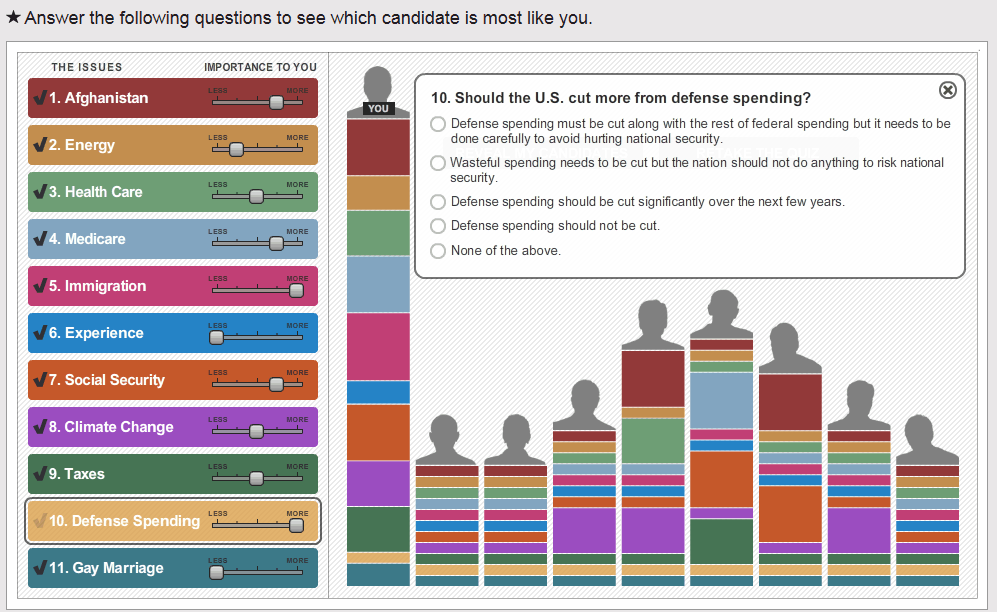
USA Today has an interesting quiz you can take that will match you up with a GOP presidential candidate. It’s here.
I didn’t find the particular questions and answers satisfying, but I imagine they’ve tried to match these up as closely as possible with the candidates’ positions. There are some interesting features to the quiz. For starters, it’s a nice piece of information architecture. The colors make it easy to track how each answer is reflected in each of the candidates’ rankings. The sliders, which let you set importance of the issues, are fun to use, and you can adjust any one of them at any time, so you can see how varying your weights effects each candidates’ score. I like that it also shows candidate “you”: this gives a feel for how closely you match up with the candidates in general. The closer the top candidate is to your bar, the closer the fit. Another nice touch: the way that the candidates are obscured by only showing silhouettes until you are done filling out the quiz. I would imagine this makes it less likely that you will try and tweak your answers and weightings to favor your favorite candidate, though if you look closely enough you can make out at least a couple of the candidates just from their silhouettes.
One final interesting note. The weightings are linear and additive. Another way to do the quiz might be to find the candidate with the best weighted geometric average. Depending on how the sliders were done, this could give you a “kill switch” to eliminate candidates who took a position opposite from yours on a single, vital issue (ie abortion). On the other hand, I suppose if you are a single issue voter you already know how each of the candidates stand on that issue.

