Lately I’ve been thinking about how to measure the fatness of the tails of a distribution. After some searching, I came across the Pareto Tail Index method. This seems to be used mostly in economics. It works by finding the decay rate of the tail. It’s complicated, both in formula and in it’s R implementation (I couldn’t get “awstindex” to run, which supposedly can be used to calculate it). The Index also has the disadvantage of being a “curve fitting” approach, where you start by assuming a particular distribution, then see which parameter gives the best fit. If this doesn’t seem morally abhorrent to you, perhaps you have a future as a high-paid econometrician.
In the past I’ve looked at how to visualize the impact of the tails on expectation, but what I really wanted was a single number to measure fatness. Poking around the interwebs, I found a more promising approach. The Mean Absolute Deviation (or MAD, not to be confused with the Median Absolute Distribution, or MAD) measures the average absolute distance between a random variable and it’s mean. Unlike the Standard Deviation (SD), the MAD contains no squared terms, which makes it less volatile to outliers.
As a result, we can use the MAD/SD ratio as a gauge of fat-tailedness. The closer the number is to zero, the fatter the tails. The closer the number is to 1 (it can never exceed 1!), the thinner the tails. For example, the normal distribution has a MAD/SD ratio of 0.7970, which happens to be the square root of 2 over pi (not a coincidence, try proving this if you rock at solving integrals).
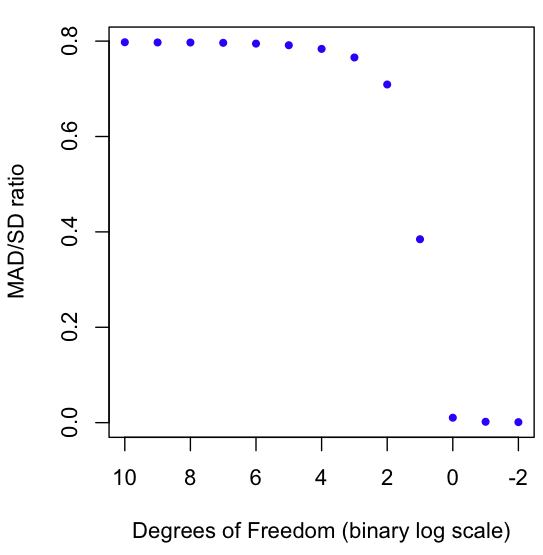
The graph at the beginning of this post shows a Monte Carlo estimation of the MAD/SD ratio for the Student T distribution as it goes from very high Degrees of Freedom (1024) to very low (1/4). You may know that the T distro converges to the Normal at high degrees of freedom (hence the result of nearly .8 for high DF), but did you know that the T distro on 1 Degree of Freedom is the same as the infamously fat-tailed Cauchy? And why stop at 1? We can keep going into fractional DFs. I’ve plotted the ratio all the way down to 1/4. As always, code in R is at the end of the post.
One more thing: there is at least one continuous distribution for which the MAD/SD ratio reaches it’s maximum possible value of one. First person to guess this maximally thin-tailed distribution gets a free copy of the comic I worked on.
# Start with a Normal, move to a Cauchy
dfs = 2^(10:-2)
results = c()
for(i in dfs) {
	x = rt(1000000,i)
	results = c(results, mean(mean(abs(x))/sd(x)))
}

# Note the wonky x-axis limit and order
plot(rev(-2:10), results, col="blue", pch=20, xlim=rev(range(-2:10)), xlab="Degrees of Freedom (binary log scale)", ylab="MAD/SD ratio")
Tags: fat tails, outliers, tails, thin tails


An interesting post and question. The central standardized fourth moment (kurtosis) is often used as a measure of the fatness of tails. In the standard moment ratio diagram, the progression of “named” symmetric distributions goes t > Normal > Triangular > Uniform > Arcsine > Beta(alpha, alpha). [Arcsine is Beta(1/2, 1/2).]
There is no continuous distribution with the smallest kurtosis because that is achieved by the Bernoulli(1/2) distribution. However, the Beta distributions of the form Beta(alpha, alpha) converges to Bernoulli(1/2) in the limit as alpha –> 0.
Thus this might be a trick question. (Are you trying to hoard those comics?) My answer is “the Beta(alpha, alpha) distribution has the thinnest tails, with alpha abritrarily small.”
You should really avoid growing your vector inside of your loop. For a simple problem like this it would be much better to preallocate ‘results’ instead of appending the new result every time.
@Rick
You’re right! The Beta goes to MAD/SD = 1 as alpha -0. Send me your mailing address from your sas email and I’ll send out a copy to you! I was thinking of the logit-normal as sigma gets big, but the distributions are basically the same at the limit, no?
I assume the only way to get to a ratio of 1 with a continuous distro is at some limit, but have no proof.
So far as Kurtosis goes, not only doesn’t it work for non-symmetrical distributions. even with symmetric ones it gets funky in oddball cases. Try this in R:
x = c(rep(0,1000),1,-1)
kurtosis(x)
and see how unstable Kurtosis is to adding another pair of 1, -1 to the end. At the extreme case of all 0′s, Kurtosis calculations choke on 0/0, whereas MAD/SD helpfully returns a 1, telling you that no tails exist.
@Dason
You are correct it’s best to initialize the vector to the size you want in advance, I usually do it that way but didn’t bother as it makes no difference for a vector so small. Best of luck with your new blog!
Nice post! It helped me. A minor point, but I didn’t realize that MAD was an ambiguous term. I just wanted to point out that the metrology (that’s measurement science, not weather) guys use the abbreviation AAD (Average Absolute Deviation). Seems like a good idea to avoid confusion.
Interesting post. Other measures of tail-fatness are investigated in Extreme Value Theory, you might want to check it out (if you don’t already know it). But I think they are very close to the Pareto tail index you mentioned.
As for the MAD/SD = 1 question, the very fact that it is less than 1 comes from the Cauchy-Schwarz inequality applied to the random variables Y=|X-EX| and Z=1. The equality occurs when these variables are exactly proportional, i.e. when X can take only 2 values symmetric w.r.t. its mean.