I should state right away that I know almost nothing about queuing theory. That’s one of the reasons I wanted to do some queuing simulations. Another reason: when I’m waiting in line at the bank, I tend to do mental calculations for how long it should take me to get served. I look at the number of tellers attending, pick an average teller session length (say one or two minutes), then come up with an average wait per person in line. For example, if there are 4 tellers and the average person takes 2 minutes to do her transaction, then new tellers should become available every 30 seconds. If I’m the 6th person in line, I should expect to wait 3 minutes before I’m attended.
However, based on my experience (the much maligned anecdotal), it often takes much longer than expected. My suspicion is that over time the teller’s get “clogged up” with the slowest people, so that even though an average person might take only 2 minutes, the people you actually see being attended right now are much more likely to be those who take a long time.
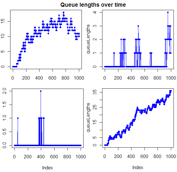
To explore this possibility, I set up a simulation in R (as usual, full source code provided at end of post). The first graph, at the beginning of this post, shows the length of queues over time for 4 runs of the simulator, all with the same configuration parameters. Often this graph was completely flat. Note though that when things get out of hand in terms of queue length, they can get way out of hand. To get a feel for how long you would have to wait, given that there is a line in front of you, I tracked how long the first person in line had to wait to be served. Given my configuration settings, this wait would be expected to last 5 intervals. It does seem to take longer than 5 intervals, though I want to tweak the model some and do more testing before I’m ready to quantify that wait.
There are, as with any models, things that make this one unrealistic. The biggest may be that people get in line with the same probability no matter how long the line is. What I need is some kind of tendency to abandon the line if it’s too long. That shouldn’t shorten the wait times for those already in line. I could make those worse. If you assume that slower people are prepared to wait longer in line, then the line is more likely to have slow people. Grandpa Jones is willing to spend an hour in line so he can chat for a while with the pretty young teller; but if the line is too long, that 50-year-old business guy will come back later to deposit his check. I would imagine that, from the bank’s perspective, this presents a tricky dilemma. The people whose time is worth the least are probably the most likely to be clogging up your tellers, upsetting the customers you care the most about (I know, I know, Bank of America cares about all of us equally, right?).
Code so far, note that run times can be very long for high intervals if the queue length gets long:
#### Code by Matt Asher. Published at StatisticsBlog.com ####
#### CONFIG ####
# Number of slots to fill
numbSlots = 5

# Total time to track
intervals = 1000

# Probability that a new person will show up during an interval
# Note, a maximum of one new person can show up during an interval
p = 0.1

# Average time each person takes at the teller, discretized exponential distribution assumed
# Times will be augmented by one, so that everyone takes at least 1 interval to serve
meanServiceTime = 25

#### INITIALIZATION ####
queueLengths = rep(0, intervals)
slots = rep(0, numbSlots)
waitTimes = c()
leavingTimes = c()
queue = list()
arrivalTimes = c()
frontOfLineWaits = c()


#### Libraries ####
# Use the proto library to treat people like objects in traditional oop
library("proto")

#### Functions ####
# R is missing a nice way to do ++, so we use this
inc <- function(x) {
  eval.parent(substitute(x <- x + 1))
}

# Main object, really a "proto" function
person <- proto(
	intervalArrived = 0,
	intervalAttended = NULL,

	# How much teller time will this person demand?
	intervalsNeeded = floor(rexp(1, 1/meanServiceTime)) + 1,
	intervalsWaited = 0,
	intervalsWaitedAtHeadOfQueue = 0,
)

#### Main loop ####
for(i in 1:intervals) {
	# Check if anyone is leaving the slots
	for(j in 1:numbSlots) {
		if(slots[j] == i) {
			# They are leaving the queue, slot to 0
			slots[j] = 0
			leavingTimes = c(leavingTimes, i)
		}
	}

	# See if a new person is to be added to the queue
	if(runif(1) < p) {
		newPerson = as.proto(person$as.list())
		newPerson$intervalArrived = i
		queue = c(queue, newPerson)
		arrivalTimes  = c(arrivalTimes, i)
	}

	# Can we place someone into a slot?
	for(j in 1:numbSlots) {
		# Is this slot free
		if(!slots[j]) {
			if(length(queue) > 0) {
				placedPerson = queue[[1]]
				slots[j] = i + placedPerson$intervalsNeeded
				waitTimes = c(waitTimes, placedPerson$intervalsWaited)
				# Only interested in these if person waited 1 or more intevals at front of line
				if(placedPerson$intervalsWaitedAtHeadOfQueue) {
					frontOfLineWaits = c(frontOfLineWaits, placedPerson$intervalsWaitedAtHeadOfQueue)
				}

				# Remove placed person from queue
				queue[[1]] = NULL
			}
		}
	}

	# Everyone left in the queue has now waited one more interval to be served
	if(length(queue)) {
		for(j in 1:length(queue)) {
			inc(queue[[j]]$intervalsWaited) # = queue[[j]]$intervalsWaited + 1
		}

		# The (possibley new) person at the front of the queue has had to wait there one more interval.
		inc(queue[[1]]$intervalsWaitedAtHeadOfQueue) # = queue[[1]]$intervalsWaitedAtHeadOfQueue + 1
	}

	# End of the interval, what is the state of things
	queueLengths[i] = length(queue);
}

#### Output ####
plot(queueLengths, type="o", col="blue", pch=20, main="Queue lengths over time", xlab="Interval", ylab="Queue length")
# plot(waitTimes, type="o", col="blue", pch=20, main="Wait times", xlab="Person", ylab="Wait time")


