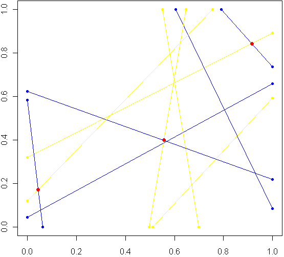
Imagine a unit square. Every side has length 1, perfectly square. Now imagine this square was really a fence, and you picked two spots at random along the fence, with uniform probability over the length of the fence. At each of these two locations, set down a special kind of cannon. Just like the light cycles from Tron, these cannons leave trails of color. To aim each cannon, pick another random point from one of the three other sides of the fence, and aim for that point.
Sometimes there will be a collision within the square, other times no. The image at top shows the results of five trials. The red dots are where the trails from a pair of cannons collided. My burning question: What is the distribution for these dots? Before reading on, try to make a guess. Where will collisions be most likely to happen?
Somewhere in the world, there lives a probabilist who could come up with a formula for the exact distribution in an hour, but that person doesn’t live in my house, so I took the Monte Carlo approach, coded in R:
# Functions to pick two points, not on the same side:
m2pt <- function(m) {
	if(m <1) {
		myPoint = c(5,m,0)
	} else if (m < 2) {
		myPoint = c(6,1,m %% 1)
	} else if (m < 3) {
		myPoint = c(7,1-(m %% 1),1)
	} else {
		myPoint = c(8,0,1-(m %% 1))
	}
	return(myPoint)
}

get2pts <- function() {
	pt1 = m2pt(runif(1,0,4))
	pt2 = m2pt(runif(1,0,4))

	# Make sure not both on the same sides. If so, keep trying
	while(pt1[1] == pt2[1]) {
		pt2 = m2pt(runif(1,0,4))
	}
	return(c(pt1[2:3],pt2[2:3]))
}

# Optional plot of every cannon fire line. Not a good idea for "iters" more than 100
#windows()
#plot(0,0,xlim=c(0,1),ylim=c(0,1),col="white")

# How many times to run the experiment
iters = 10000

# Track where the intersections occur
interx = c()
intery = c()

for(i in 1:iters) {
	can1 = get2pts()
	can2 = get2pts()

	# Optional plot of every cannon fire line. Not a good idea for "iters" more than 100
	#points(c(can1[1],can1[3]),c(can1[2],can1[4]),pch=20,col="yellow")
	#segments(can1[1],can1[2],can1[3],can1[4],pch=20,col="yellow",lwd=1.5)
	#points(c(can2[1],can2[3]),c(can2[2],can2[4]),pch=20,col="blue")
	#segments(can2[1],can2[2],can2[3],can2[4],pch=20,col="blue",lwd=1.5)

	# See if there is a point of intersection, find it.
	toSolve = matrix(c( can1[3]-can1[1], can2[3]-can2[1], can1[4]-can1[2], can2[4]-can2[2]),byrow=T,ncol=2)
	paras = solve(toSolve, c( can2[1]-can1[1], can2[2]-can1[2]))

	solution = c(can1[1] + paras[1]*(can1[3]-can1[1]), can1[2] + paras[1]*(can1[4]-can1[2]))

	# Was the collision in the square
	if(min(solution) > 0 && max(solution) < 1) {
		# Optional plot of red dots
		# points(solution[1],solution[2],pch=20,col="red",cex=1.5)

		# if this intersection is in square, plot it, add it to list of intersections
		interx = c(interx, solution[1])
		intery = c(intery, solution[2])
	}
}

windows()
plot(interx, intery, pch=20,col="blue",xlim=c(0,1),ylim=c(0,1))
After carefully writing and debugging much more code than I expected, I ran a trial with several thousand cannon fires and plotted just the collisions. Here is what I saw:
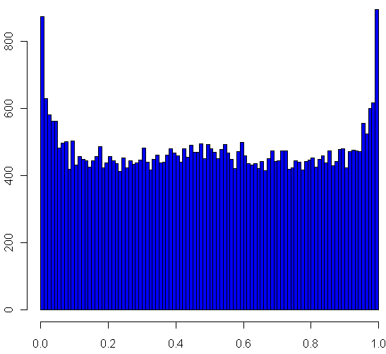
Looks pretty uniform, doesn't it? If it is, I will have gone a very long way just to replicate the bi-variate uniform distribution. My own original guess was that most collisions, if they happened in the square, would be towards the middle. Clearly this wasn't the case. Looks can be deceiving, though, so I checked a histogram of the x's (no need to check the y's, by symmetry they have the same distribution):
Very interesting, no? The area near the edges appears more likely to have a collision, with an overall rounded bowl shape to the curve. The great thing about Monte Carlo simulations is that if something unexpected happens, you can always run it again with more trials. Here I changed "iters" to 100,000, ran the code again, and plotted the histogram.
hist(interx, breaks=100, col="blue",xlab="x",main="Histogram of the x's")
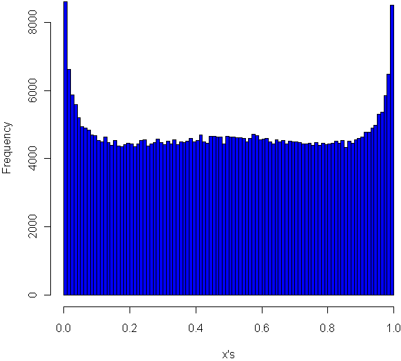
Now its clear that the distribution spikes way up near the edges, and appears to be essentially flat for most of the middle area. It seems like it may even go up slightly at the very middle. Just to be sure, I ran a trial with one million iterations:
Now it definitely looks like a small upward bulge in the middle, though to be sure I would have to do run some statistical tests or use an even larger Monte Carlo sample, and given how inefficient my code is, that could take the better part of a week to run. So for today I'll leave it at that.
One final statistic of note: During my run of one million iterations, 47.22% of all collisions happened inside the box. What do you think, is the true, theoretical ratio of collisions within the box a rational number?


Neat example, Matt. I was misled by the first plot, and thought you’d be looking at a whole bunch of shots at once.
It looks like the proportion of experiments with collisions in the box is 0.5.
Hi Ken,
Good point about the plot. If there were more lines you’d see that only a few of the overlaps led to red collisions (maybe x’s would be better?), but that would look messy.
A proportion of 0.5 would have a nice feel to it, and it’s not that far from the approx. 47% I got by Monte Carlo, but that was with 1 million trials. My quick calculations show that to be about 6 sigma (normal approx to binomial), which is to say unlikely.
Cheers,
Matt
3 / (2*pi) ??
See also Buffon’s Needle.
Just realized I was off by an order of magnitude in my comment. If the true ratio was .5 then what I observed would be closer to a 60 sigma event!
If the true ratio was 3 / (2*pi) = 47.75% that’s much closer to the test results, but would still mean my test deviated by 10 standard deviations from the mean. A good thought to use Buffon’s Needle as a guide though.
Answer is 17/36 = 0.4722 recurring (compute by integration of probability conditional on end points of first line, distinguishing where ends of first line on opposite sides (1/3) and on adjacent sides (2/3))
Relevant conditional probabilities are [4+2xy-x-y]/6 for opposite sides (taking x and y as distances of points from opposite corners of square) and [3x+3y-2xy]/6 for adjacent sides (taking x and y as distances from common corner).
Rest left as exercise.
Actually, the true rate is 17/36, this correspond exactly to 47.22 %. Here is a proof : http://dl.dropbox.com/u/1850029/cannon.pdf
Ah – pleased to see that histogram 🙂 My guess (really just an extremely vague intuition) was that the behaviour of the system would be similar to the distribution time spent on either side of the origin by a 1D random walk. You see this used as a teaching example where there are two players; Alice pays Bob a penny for each walk step above the origin, while Bob pays Alice for each walk step below (with some tie-break convention for a step at 0). For a game with N steps, a player is most likely to either win N times or o times and least likely to win a middling number of times.
Great to see all the effort that went into finding the true solution! So people know I have to approve all comments by new commenters first (to filter spam that isn’t caught by the filter, ugh!). As a result none of the last 3 posters saw each other’s comments before posting.
I’ll post a followup to this blog post very soon.
Coming very late into the discussion, I confirm the 17/36 result (I did the computation when driving across France the day before yesterday but could not post the outcome). Now the shape of the histogram is suggesting an arcsine distribution, as in the percentage of positive gains along a very long series of head and tail games (Feller, 1970, volume 1). another point already made in the comments…
Following my previous comment, I looked at the distributions of the collision coordinates, conditional on the location of the endpoints of the segments on the unit square. Depending on those locations, a fit by a Beta(a,a), a Beta(1,a) or a Beta(a,1) is rather accurate. I would thus suggest that the histogram observed above is in fact a mixture of Beta distributions.
@xi’an
It’s certainly possible to generate a histogram that looks a lot like the final one using a mixture of Betas. Just playing around I came up with this:
hist(c(rbeta(100000,.5,.5),rbeta(20000,3.5,3.5)),breaks=100,col=”blue”)
which looks much like the final histogram. Though I suppose you could have “mixed in” just about any symmetric, unimodal distribution to get the small hump in the middle.
Nice problem! Still thinking about the spatial distribution…
There’s a really quick way to get the 17/36 figure with no integration (sorry if this is a repeat comment) — first find the probabilities that the endpoints are on a certain configuration of sides; and then for any given configuration of sides, you can see that the probability of collision is always either 0, 1, or 1/2.
Hi,
As part of a code I’m writing to study seismic fault orientations, I had to generate a set of random segments ( each x,y coordinate of each segment tip being drawn from an uniform distribution so that they all lie within the square). Then I divided the square in square cells and counted, for each cell, the number of rays passing through it. This gives me a density map. For some reason, I was expecting an uniform coverage of that square surface, but it turned out that I obtained a distribution which definitely looks like the one you obtain in your experiment, without the peaks on each edge of the square though. The density function I obtain exhibits a slight bulge, with a maximum density in the middle of the square, and minimum densities close to the square’s edges. The main difference between my experiment and yours is that my segments start and end anywhere within the square, and not only on its edges. I also think we’re not exactly counting the same thing : counting the number of times a cell is hit by a segment is actually a bit different from counting the number of times segments have intersected each other within that particular cell (for instance three parallel segments can hit a cell, but they don’t intersect each other). I have to say that I was a bit puzzled by such a distribution and that’s how, after a little bit of time wandering on the web, I ended up on this page. And I have a question : is there a way to get an analytic estimate of the shape of such a density function?