Probability and statistics blog

It’s 1943 and you work for the good guys. A handful of German tanks have been captured, and each one has a serial number. This is back when serial numbers were still presumed to come in serial, one right after the other. Given your collection of numbered tanks, and assuming that any existing tank was just as likely to be captured as any other, how many tanks would you guess that the Krauts have?

By luck, you have a time machine, so you jump forward in time, check out the Wikipedia entry, and copy down the formula [latex]\hat{N} = \frac{k+1}{k} m – 1 = m + \frac{m}{k} – 1[/latex], noting that [latex]m[/latex] should be replaced with the highest serial number encountered, while [latex]k[/latex] represents the number of tanks captured. Reading on, you see that Wikipedia has provided a rare nugget of actual understanding for a formula. This estimate represents “the sample maximum plus the average gap between observations in the sample”.

So you’re done, right? Just plug in to the formula, hand in your estimate to the commanding officer, go enjoy some R&R. Not so fast. Here at StatisticsBlog.com, nothing is believed to work until it passes the Monte Carlo test. To test out the formula I coded a simulation in R:

# Function to estimate maximum from sample "samp"
gTank <- function(samp) {
	 max(samp) + max(samp)/length(samp) - 1
}

# A blank log-log plot to get us started
plot(100,100, xlim=c(100,10^7), ylim=c(100,10^7), log="xy",pch=".",col="white",frame.plot=F,xlab="True value",ylab="Predicted")

# Let's track residuals
trueTops = c()
resids = c()
sampleTops = c()

x = runif(100,2,6)
for(i in x) {
	trueTop = 10^i
	for(j in 1:50) {
		observeds = sample(1:trueTop, 20) # No replacement here
		guess = gTank(observeds)

		# Plot the true value vs the predicted one
		points(trueTop,guess,pch=".",col="blue",cex=2) 

		trueTops = c(trueTops, trueTop)
		resids = c(resids, trueTop - guess)
		sampleTops = c(sampleTops, max(observeds))
	}
}

# Platonic line of perfectly placed predictions
lines(c(100,10^6),c(100,10^6),lty = "dashed",col="gray",lwd=1)

# Plot residuals too
windows()
plot(trueTops,log="x",resids,pch=20,col="blue",xlab="True value",ylab="Residual",main="Residuals plot")
abline(h=0)

mean(abs(resids))
mean(trueTops-sampleTops)

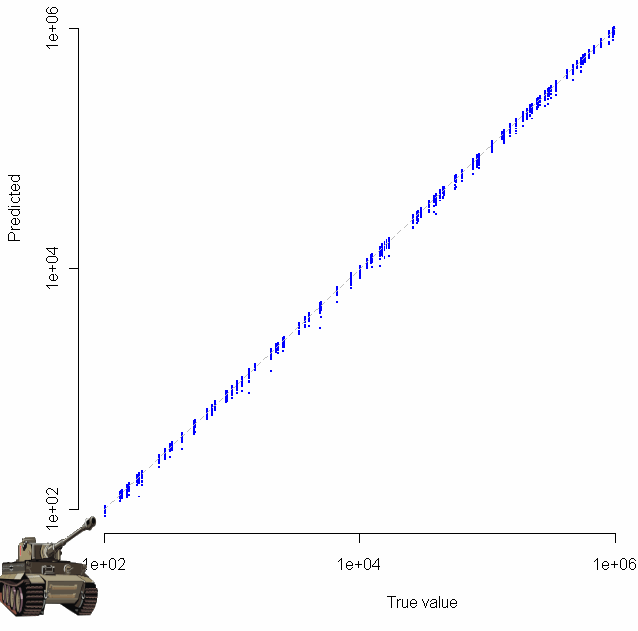
Which produces the following log-log plot:

Gratuitous clip art was added with the “chartJunk()” function.

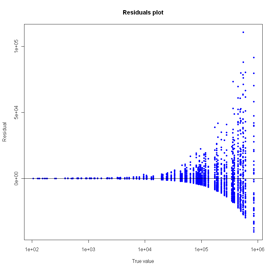
Looks pretty good, no? Especially given that the sample size for each of these tests was just 20. To make sure everything was OK, I plotted the residuals as well:

Make sure to click on the images above to see larger versions. Bigger really is better when it comes to viewing charts. Looks good too, no?

So, German tank problem estimate? Confirmed. Just don’t dig too deep into the assumption that all tanks had an equal chance of being captured; common sense goes against that one (ask yourself if there might be a relationship between length of time a tank is in the field of battle and the likelihood it will be captured).

Speaking of likelihood… this problem gives a nice example of how maximum likelihood estimation (MLE) can fail in spectacular form, like a bomb whose innards have been replaced by sawdust (alright, I promise, last military analogy). The MLE for the number of German tanks is the highest serial number observed. This is because MLE works backwards, finding the parameter which makes our observation most likely in terms of joint conditional probability. As a result, the MLE for this problem is not only biased (since it will always be less than or equal to the true number of tanks), but dumb as well. How likely is it (in the common sense usage of the term) that your captured tanks will include the highest-numbered one? If the distribution is truly uniform, the chance that you have to top one is [latex]\frac{k}N[/latex] where [latex]N[/latex] is the true, unknown number of tanks. You don’t know [latex]N[/latex], but you do know that it’s at least [latex]m[/latex] (the highest number observed). For small samples, where [latex]k << m[/latex], the probability that you have captured the very top-numbered tank is quite small indeed, no larger than [latex]\frac{k}m[/latex] at best.

Just how bad is the MLE? I compared the mean absolute residuals from the two different methods. Using the formula from at the beginning of this post gives 6,047. Using MLE, the average residual was 8,175, or 35% worse. Standard deviation for the MLE method is also higher, by about 27%. Back to boot camp for the MLE. (I know, I know, I promised).

Tags: german tank problem, mle, r

This entry was posted on Tuesday, May 25th, 2010 at 11:49 am and is filed under feature, r, stats. You can follow any comments to this entry through the RSS 2.0 feed. Both comments and pings are currently closed.